电磁场耦合仿真-主题078_电磁场拓扑优化-电磁场拓扑优化

第七十八篇：电磁场拓扑优化

摘要

电磁场拓扑优化是一种先进的结构设计方法，通过在给定设计空间内优化材料分布，实现电磁器件性能的最优化。本主题系统介绍拓扑优化的基本理论、数学模型、数值算法以及在电磁场设计中的应用。重点阐述SIMP（固体各向同性材料惩罚）方法、水平集方法、进化结构优化（ESO）等主流拓扑优化算法，探讨电磁场目标函数（如S参数、辐射效率、场均匀性等）的灵敏度分析方法。通过Python实现微波器件、天线结构、电磁屏蔽等典型应用的拓扑优化设计，展示从初始设计到优化结构的完整演化过程，为电磁器件的轻量化、高性能化设计提供理论指导和工程实践方法。

关键词

拓扑优化，SIMP方法，水平集方法，进化结构优化，灵敏度分析，材料插值，滤波技术，电磁器件设计

1. 拓扑优化基础理论

1.1 拓扑优化概述

拓扑优化的定义：

拓扑优化是在给定设计域、边界条件和约束条件下，寻找最优材料分布的结构优化方法。与尺寸优化和形状优化不同，拓扑优化可以改变结构的连通性和拓扑形式。

数学描述：

$$\underset{\rho }{\min }J(\rho )\text{s.t.}{g}_i(\rho )\le 0,i=1,2,\dots ,m$$

其中 $\rho$ 为材料密度分布，$J$ 为目标函数，$g_i$ 为约束条件。

设计变量：

在离散化框架下，设计变量为每个单元的材料密度：

$${\rho }_e\in [0,1],e=1,2,\dots ,N$$

其中 ${\rho }_e=0$ 表示空（无材料），${\rho }_e=1$ 表示实（满材料）。

1.2 拓扑优化与电磁场设计

电磁场设计中的拓扑优化：

将拓扑优化应用于电磁场设计，需要建立电磁场响应与材料分布之间的关系：

材料属性插值：

电磁参数（介电常数、磁导率、电导率）与材料密度的关系：

$$\epsilon (\rho )={\epsilon }_{min}+{\rho }^p({\epsilon }_{max}-{\epsilon }_{min})$$
$$\mu (\rho )={\mu }_{min}+{\rho }^p({\mu }_{max}-{\mu }_{min})$$

其中 $p$ 为惩罚因子，通常 $p\ge 3$。

电磁场控制方程：

考虑材料分布的麦克斯韦方程组：

$$\nabla \times \left(\frac{1}{\mu (\rho )}\nabla \times \mathbf{E}\right)-{\omega }^2\epsilon (\rho )\mathbf{E}=-j\omega \mathbf{J}$$

1.3 拓扑优化的优势

2. 拓扑优化数学模型

2.1 SIMP方法

固体各向同性材料惩罚模型（SIMP: Solid Isotropic Material with Penalization）：

SIMP方法通过引入惩罚因子，使中间密度材料变得不经济：

$$E(\rho )=E_{min}+{\rho }^p(E_{max}-E_{min})$$

其中 $p>1$ 为惩罚因子，通常取 $p=3$。

优化问题表述：

$$\underset{\rho }{\min }J(\mathbf{E}(\rho ))$$
$$\text{s.t.}\nabla \times \left(\frac{1}{\mu (\rho )}\nabla \times \mathbf{E}\right)-{\omega }^2\epsilon (\rho )\mathbf{E}=-j\omega \mathbf{J}$$
$$0<{\rho }_{min}\le {\rho }_e\le 1,e=1,2,\dots ,N$$
$$V(\rho )=\sum _e{\rho }_e{v}_e\le V^{\ast }$$

灵敏度分析：

目标函数对设计变量的灵敏度：

$$\frac{\partial J}{\partial {\rho }_e}=\frac{\partial J}{\partial \epsilon }\frac{\partial \epsilon }{\partial {\rho }_e}+\frac{\partial J}{\partial \mu }\frac{\partial \mu }{\partial {\rho }_e}$$

其中：

$$\frac{\partial \epsilon }{\partial {\rho }_e}=p{\rho }_e^{p-1}({\epsilon }_{max}-{\epsilon }_{min})$$

2.2 水平集方法

水平集函数：

用隐式函数 $\varphi (\mathbf{x})$ 描述结构边界：

$$\{\begin{array}{ll}\varphi (\mathbf{x})>0& \text{材料域}\\ \varphi (\mathbf{x})=0& \text{边界}\\ \varphi (\mathbf{x})<0& \text{空域}\end{array}$$

Hamilton-Jacobi方程：

水平集函数的演化方程：

$$\frac{\partial \varphi }{\partial t}+V_n|\nabla \varphi |=0$$

其中 $V_n$ 为法向速度，由灵敏度决定：

$$V_n=-\frac{\partial J}{\partial \varphi }$$

材料属性表示：

$$\epsilon (\varphi )={\epsilon }_{min}+H(\varphi )({\epsilon }_{max}-{\epsilon }_{min})$$

其中 $H(\varphi )$ 为Heaviside函数：

$$H(\varphi )=\{\begin{array}{ll}1& \varphi \ge 0\\ 0& \varphi <0\end{array}$$

2.3 进化结构优化（ESO）

ESO基本原理：

逐步移除对目标函数贡献最小的材料单元：

灵敏度阈值：

$${\alpha }_{th}={\alpha }_{min}+r_i({\alpha }_{max}-{\alpha }_{min})$$

其中 $r_i$ 为进化率，随迭代逐步增加。

双向ESO（BESO）：

同时允许材料添加和移除：

• 移除：灵敏度低于下限的单元
• 添加：灵敏度高于上限的空单元

3. 数值实现技术

3.1 有限元离散

设计域离散：

将设计域离散为有限元网格，每个单元具有独立的材料密度：

$$\Omega =\bigcup _{e=1}^N{\Omega }_e$$

单元矩阵组装：

全局系统矩阵：

$$\mathbf{K}=\sum _e{\rho }_e^p{\mathbf{K}}_e$$

其中 ${\mathbf{K}}_e$ 为单元刚度矩阵。

3.2 滤波技术

密度滤波：

解决棋盘格问题和网格依赖性：

$${\tilde{\rho }}_e=\frac{{\sum }_i{w}_{ei}{\rho }_i}{{\sum }_i{w}_{ei}}$$

其中权重函数：

$$w_{ei}=\max (0,r_{min}-r_{ei})$$

$r_{min}$ 为滤波半径，$r_{ei}$ 为单元中心距离。

灵敏度滤波：

$$\frac{\partial \tilde{J}}{\partial {\rho }_e}=\frac{{\sum }_i{w}_{ei}\frac{\partial J}{\partial {\rho }_i}}{{\rho }_e{\sum }_i{w}_{ei}}$$

3.3 投影技术

Heaviside投影：

获得清晰的0/1材料分布：

$${\bar{\rho }}_e=\frac{\tanh (\beta \eta )+\tanh (\beta ({\tilde{\rho }}_e-\eta ))}{\tanh (\beta \eta )+\tanh (\beta (1-\eta ))}$$

其中 $\beta$ 控制投影陡峭度，$\eta$ 为投影阈值。

4. 电磁场目标函数

4.1 S参数优化

目标函数：

最小化反射系数或最大化传输系数：

$$J=|S_{11}{|}^2\text{或}J=-|S_{21}{|}^2$$

灵敏度推导：

利用伴随变量法：

$$\frac{\partial J}{\partial {\rho }_e}=2\Re \left\{{\mathbf{E}}^T\frac{\partial \mathbf{K}}{\partial {\rho }_e}{\mathbf{E}}_{adj}\right\}$$

其中 ${\mathbf{E}}_{adj}$ 为伴随场。

4.2 辐射特性优化

天线增益最大化：

$$J=-G({\theta }_0,{\varphi }_0)$$

其中 $G$ 为特定方向的增益。

辐射效率最大化：

$$J=-\frac{P_{rad}}{P_{in}}$$

4.3 场均匀性优化

场分布均匀性：

$$J={\int }_{{\Omega }_{target}}|E-E_{target}{|}^{2}d\Omega$$

场集中性：

$$J=-{\int }_{{\Omega }_{target}}|E{|}^{2}d\Omega$$

5. 优化算法

5.1 优化准则法（OC）

更新格式：

$${\rho }_e^{new}=\{\begin{array}{ll}\max ({\rho }_{min},{\rho }_e-m)& \text{if }{\rho }_e{B}_e^{\eta }\le \max ({\rho }_{min},{\rho }_e-m)\\ \min (1,{\rho }_e+m)& \text{if }{\rho }_e{B}_e^{\eta }\ge \min (1,{\rho }_e+m)\\ {\rho }_e{B}_e^{\eta }& \text{otherwise}\end{array}$$

其中 $B_e$ 为灵敏度比值，$m$ 为移动限制。

5.2 序列线性规划（SLP）

线性近似：

$$J(\rho +\Delta \rho )\approx J(\rho )+\nabla J^T\Delta \rho$$

约束线性化：

$$g_i(\rho )+\nabla g_i^T\Delta \rho \le 0$$

5.3 序列二次规划（SQP）

二次近似：

$$\underset{\Delta \rho }{\min }\nabla J^T\Delta \rho +\frac{1}{2}\Delta {\rho }^T\mathbf{H}\Delta \rho$$
$$\text{s.t.}{g}_i+\nabla g_i^T\Delta \rho \le 0$$

其中 $\mathbf{H}$ 为Hessian矩阵或其近似。

6. 工程应用

6.1 微波器件设计

滤波器拓扑优化：

• 优化谐振腔结构
• 实现特定的频率响应
• 减小器件尺寸

功分器设计：

• 优化功率分配网络
• 改善阻抗匹配
• 减小插入损耗

6.2 天线设计

天线结构优化：

• 优化天线辐射单元形状
• 提高增益和带宽
• 实现多频段工作

超表面设计：

• 优化单元结构
• 实现波束调控
• 设计聚焦透镜

6.3 电磁屏蔽

屏蔽罩设计：

• 优化开孔位置和形状
• 平衡屏蔽效能和散热
• 最小化重量

7. 案例研究

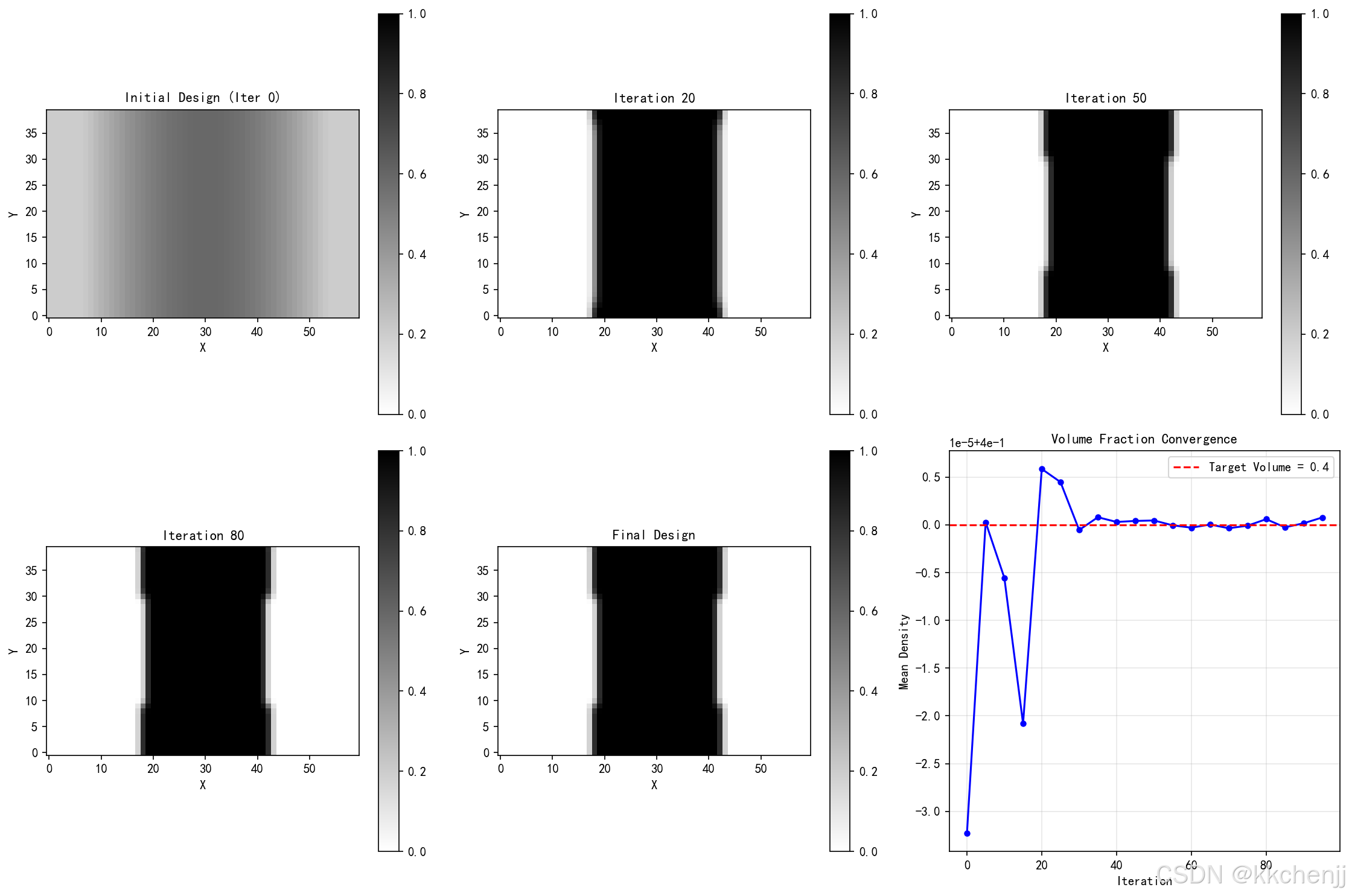
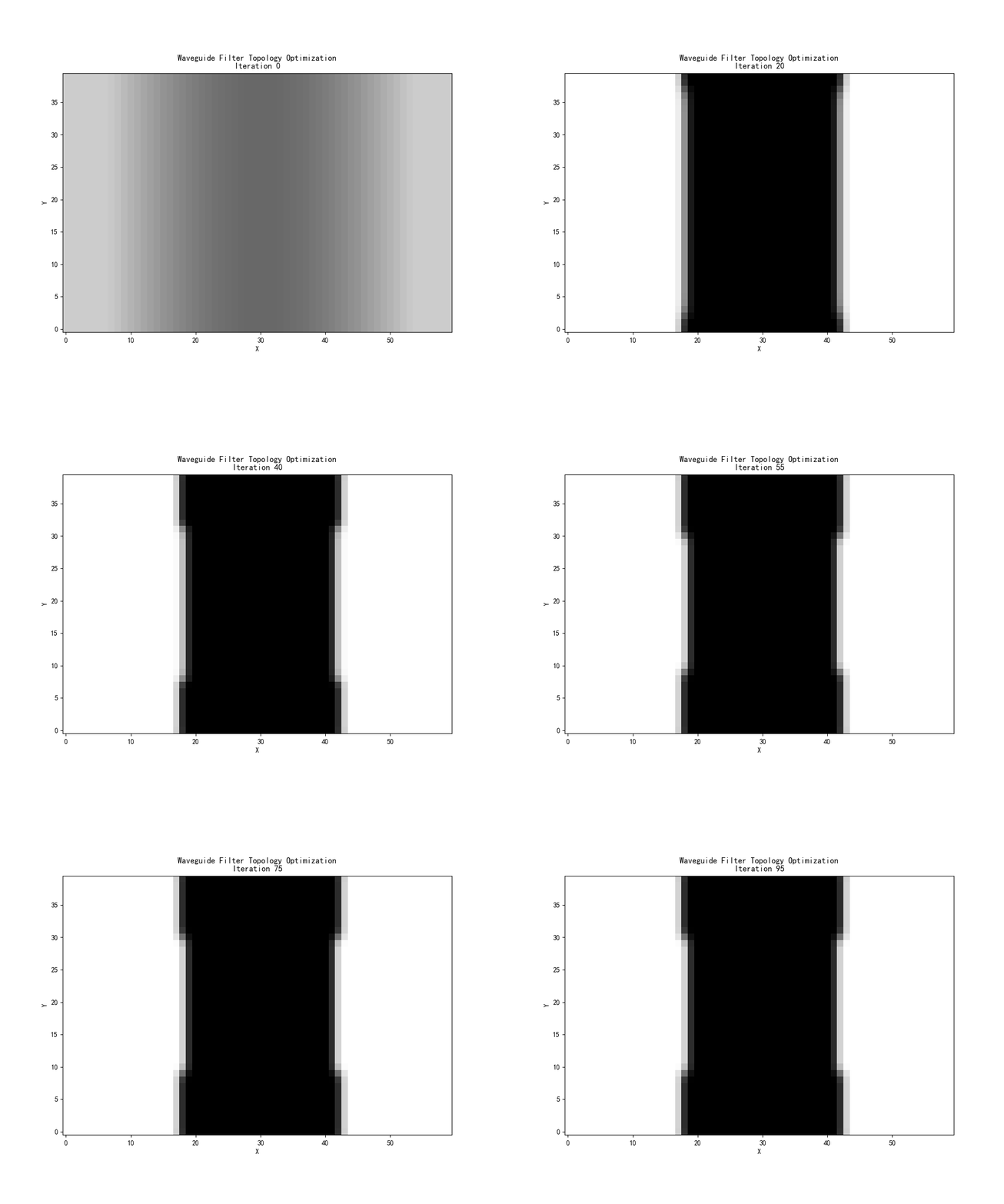
7.1 案例1：波导滤波器拓扑优化（含GIF动画）

优化波导腔体结构，实现特定的带通滤波特性。

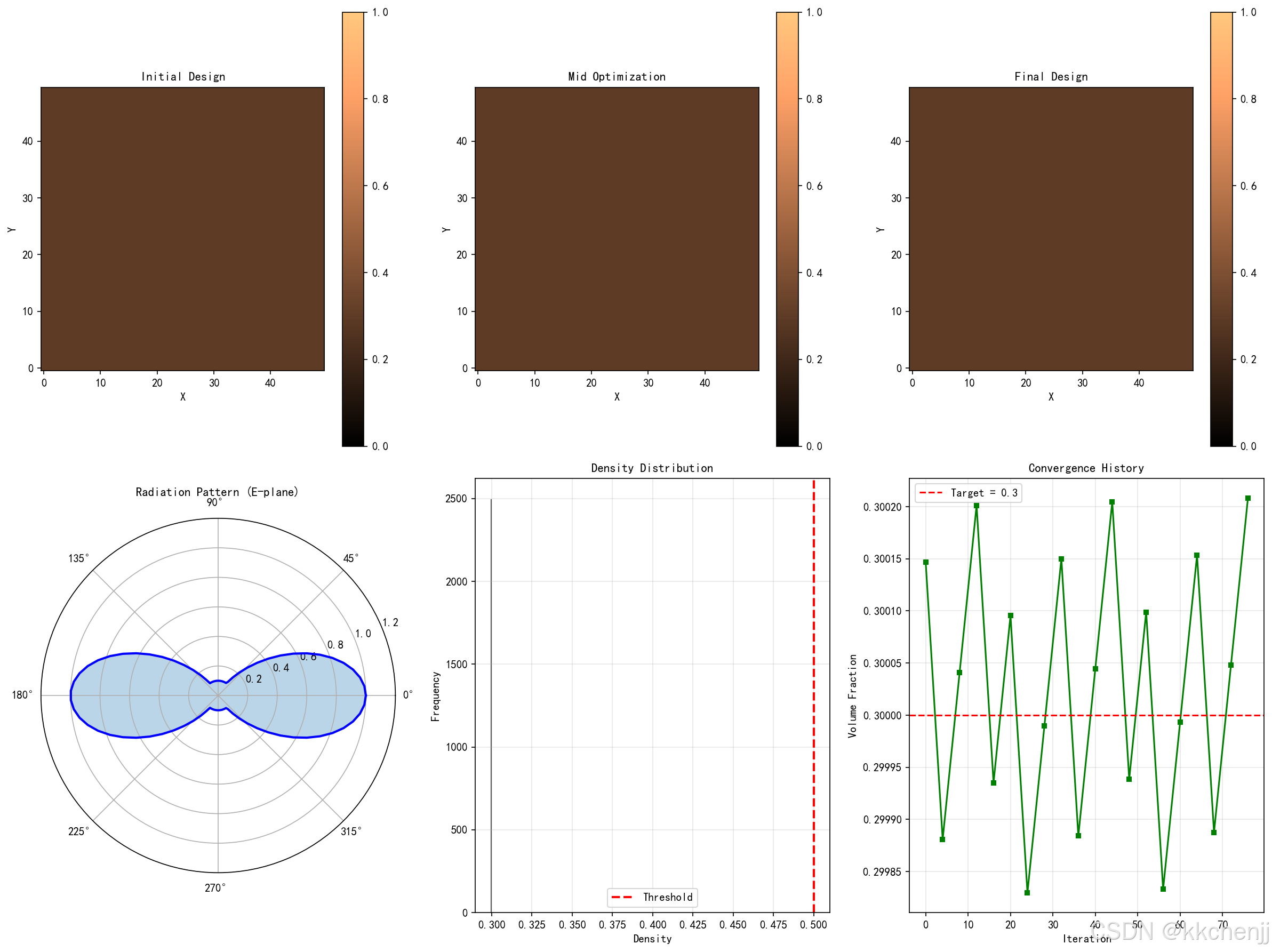
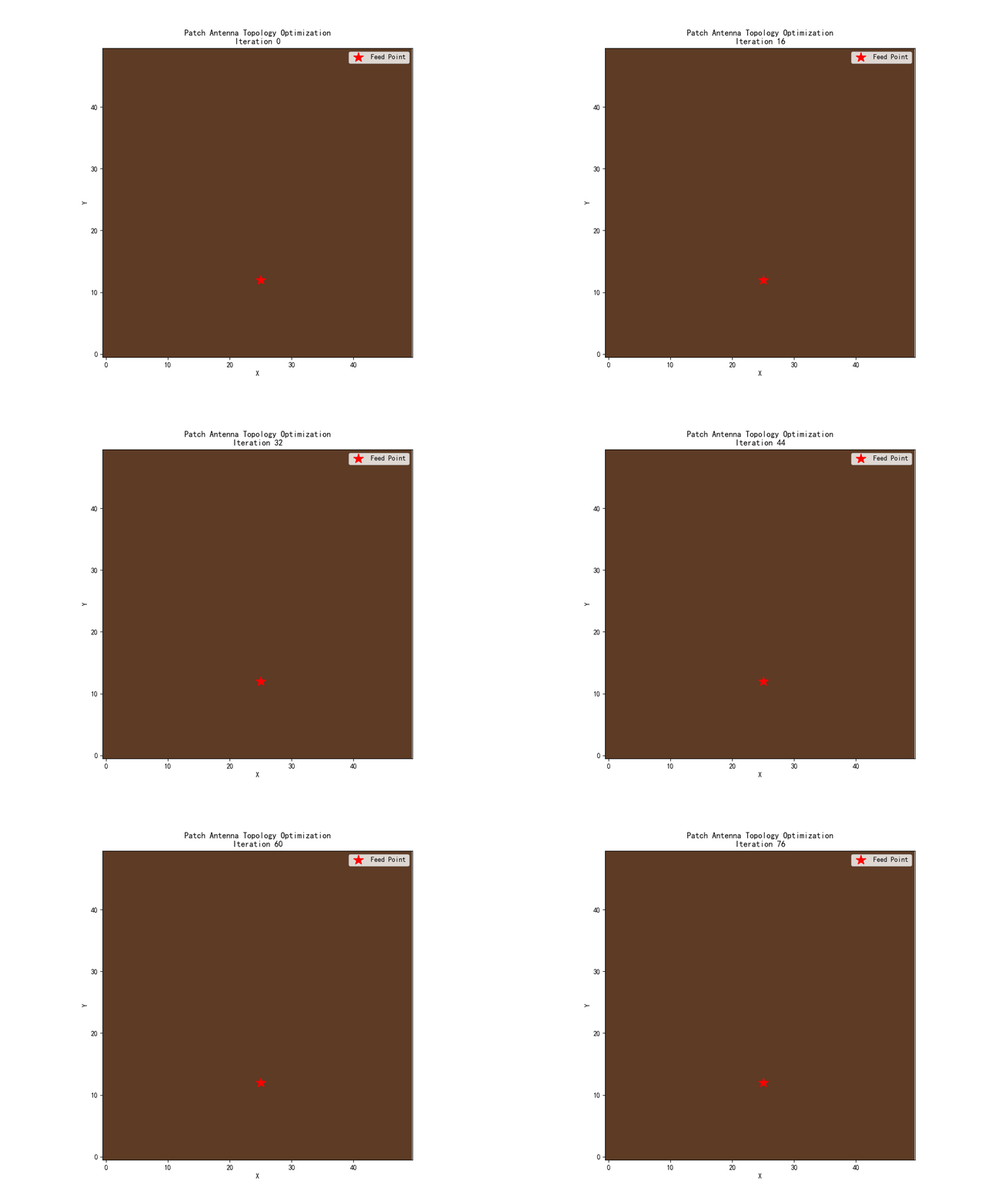
7.2 案例2：贴片天线拓扑优化（含GIF动画）

优化贴片天线的金属分布，提高辐射效率和增益。

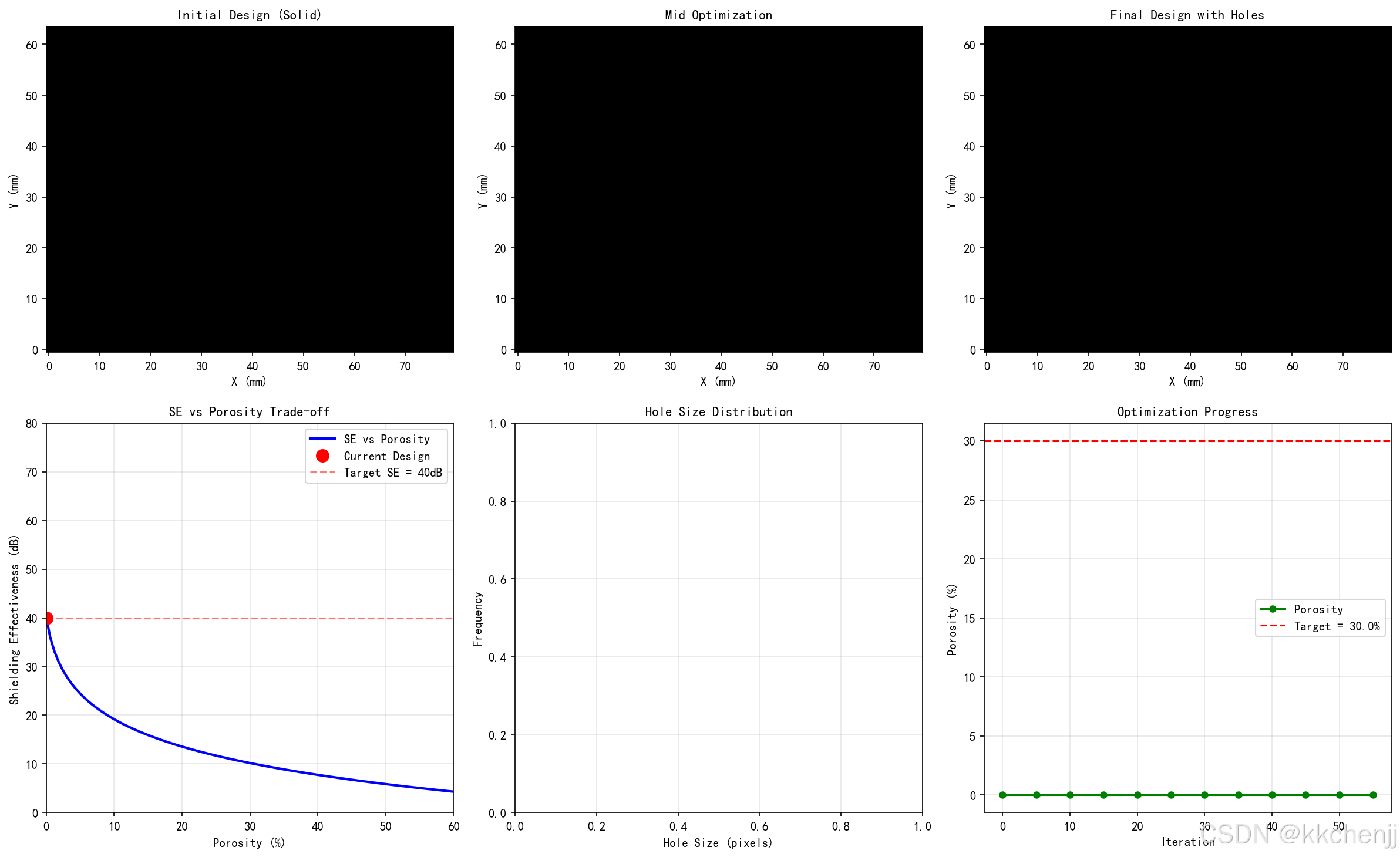
7.3 案例3：电磁屏蔽罩开孔优化

在屏蔽效能约束下，优化散热孔的布局和形状。

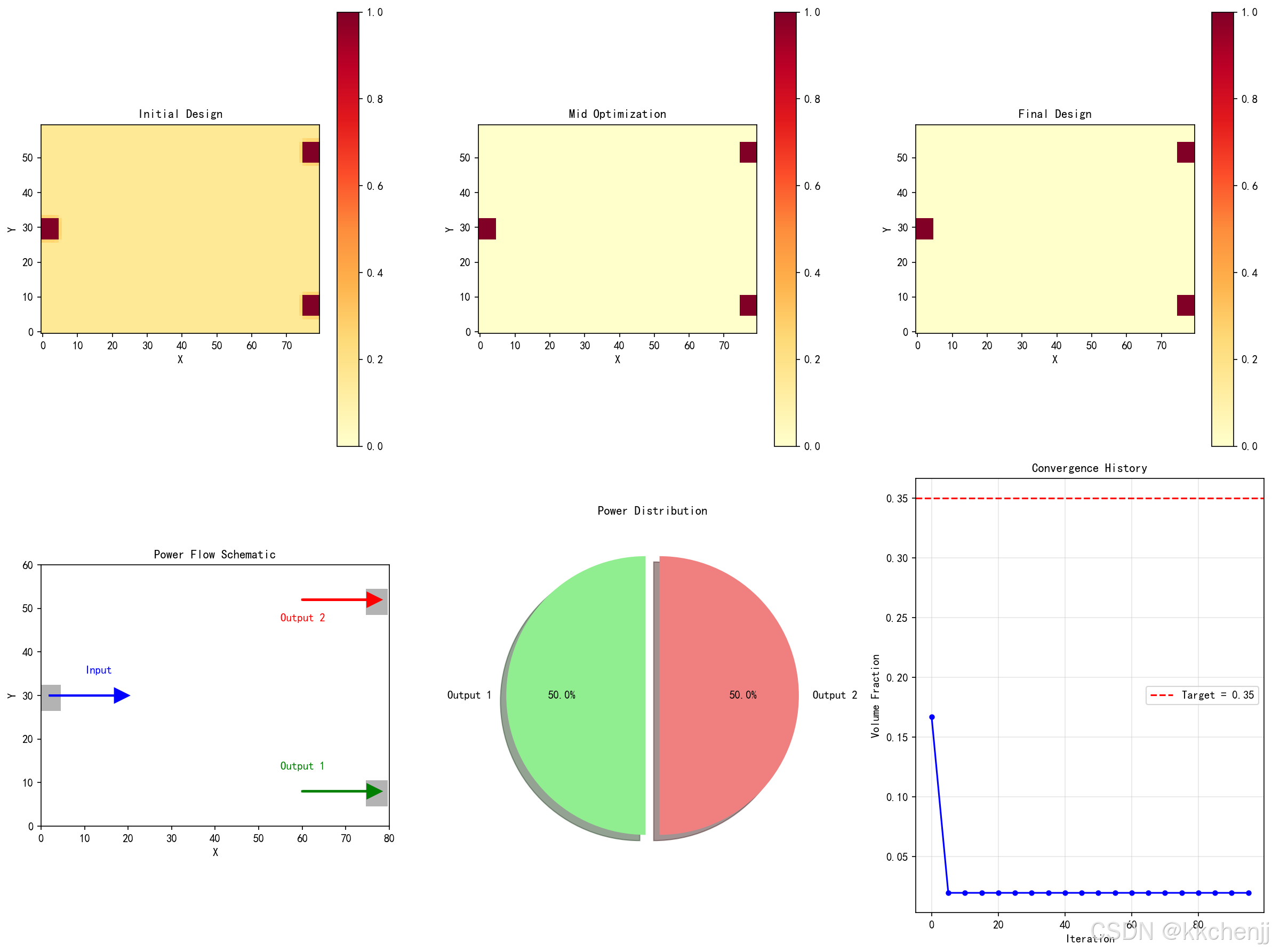
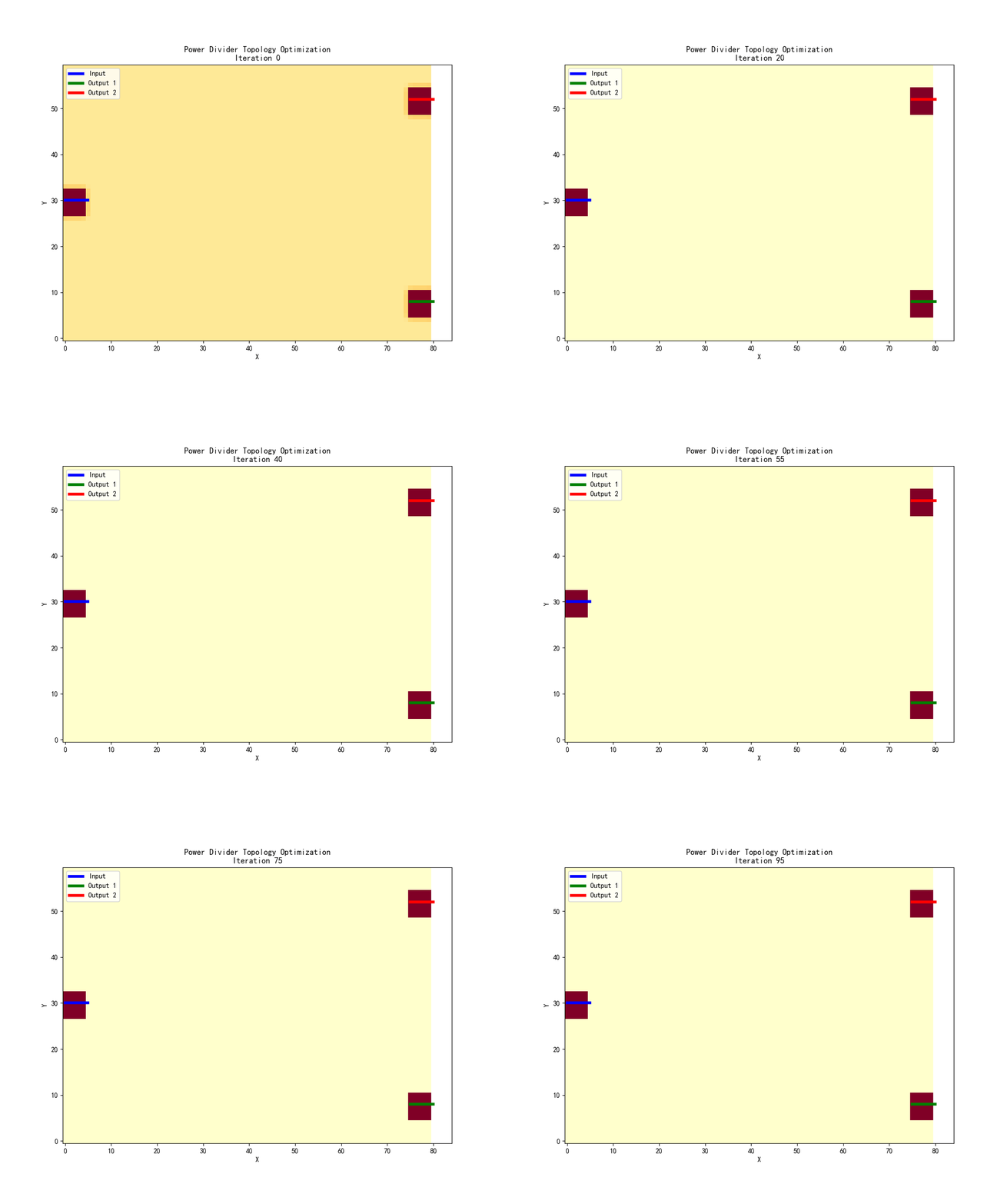
7.4 案例4：功分器拓扑优化（含GIF动画）

优化微带功分器的结构，实现功率均匀分配。

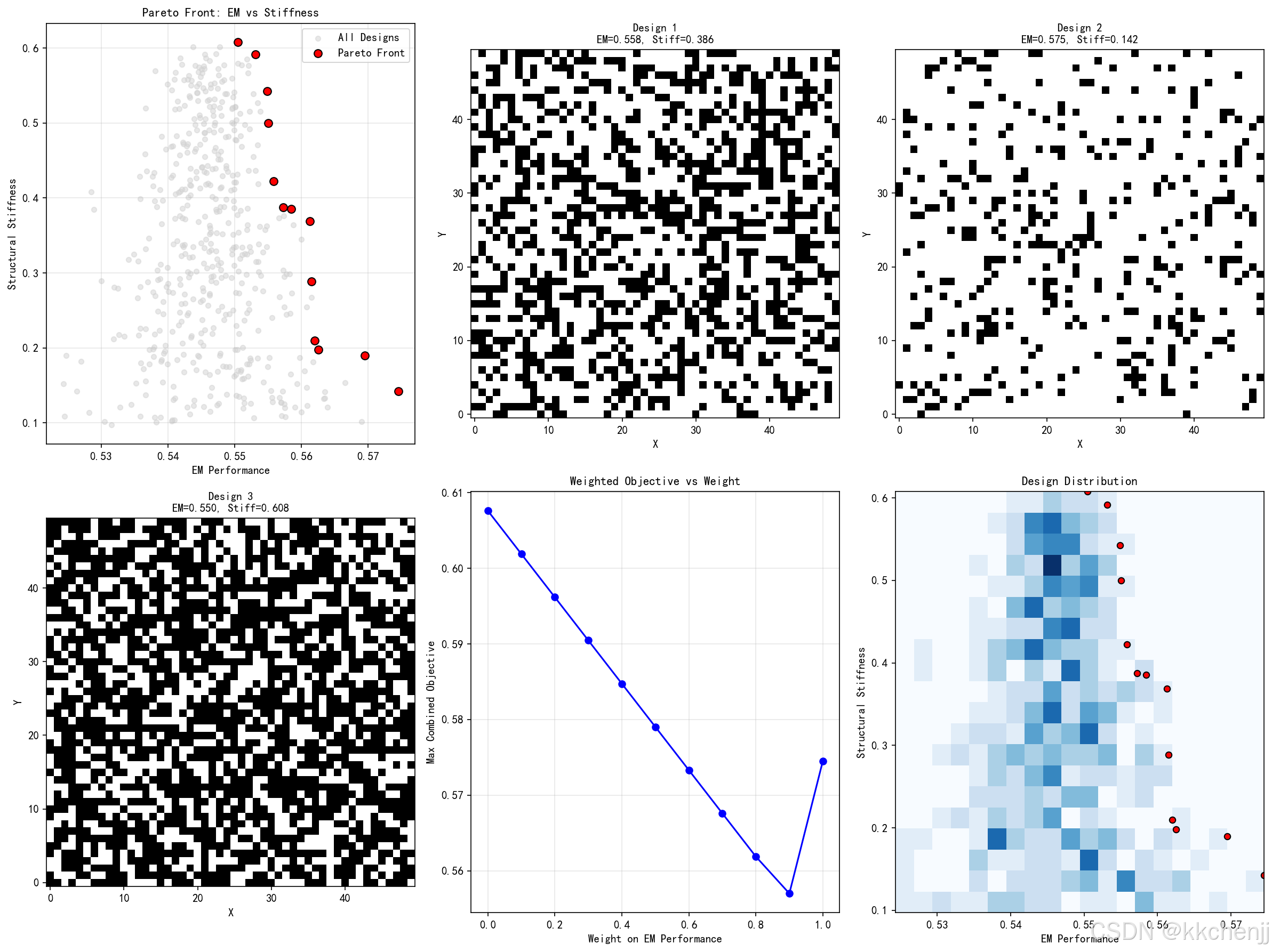
7.5 案例5：多目标拓扑优化

同时优化电磁性能和结构刚度，实现多功能设计。

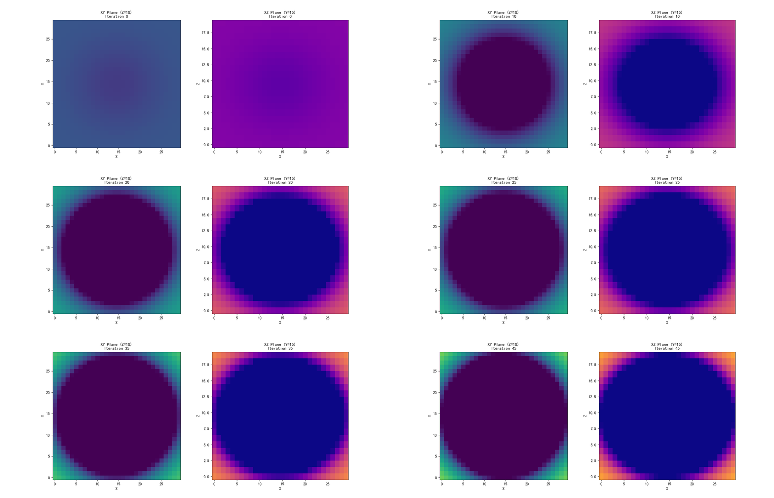
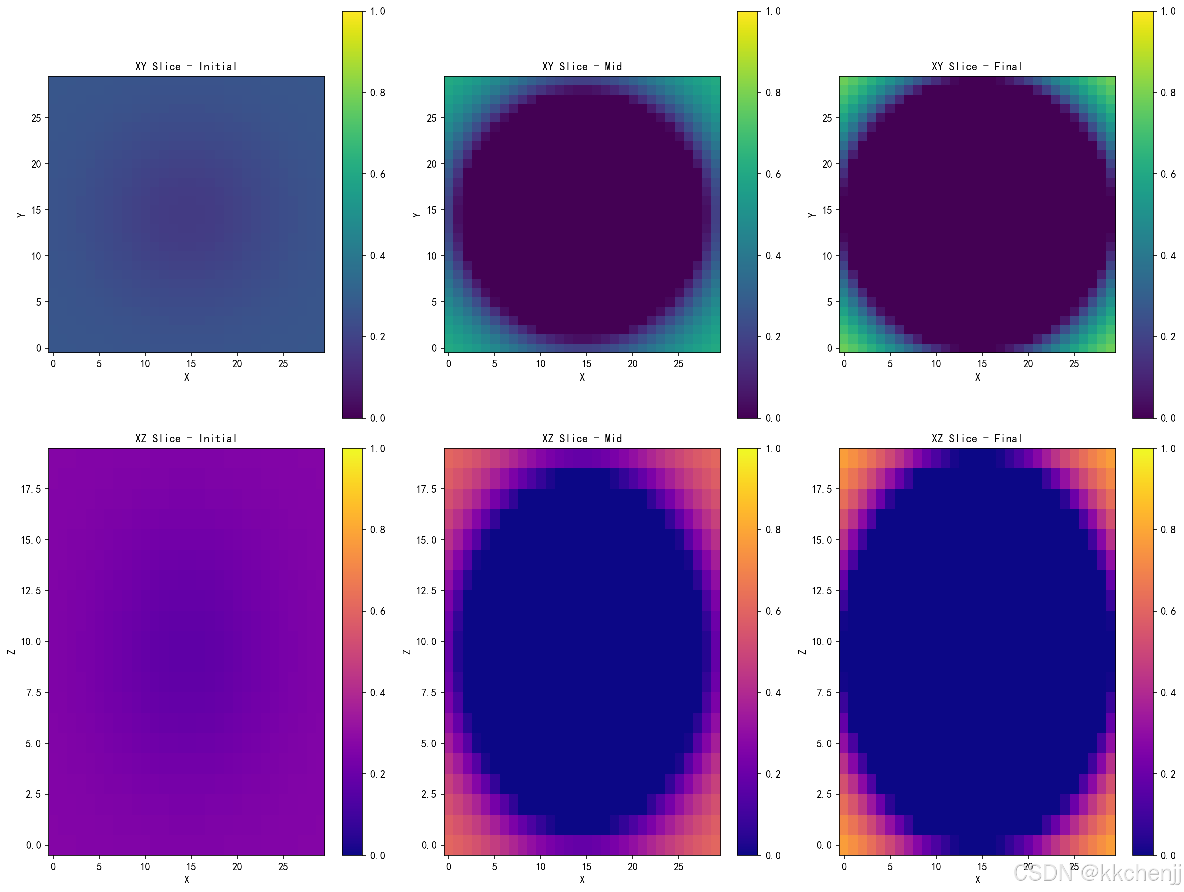
7.6 案例6：三维拓扑优化（含GIF动画）

展示三维电磁器件的拓扑优化过程和结果。

8. 结果分析与讨论

8.1 优化结果验证

• 全波仿真验证
• 实验测试对比
• 制造可行性评估

8.2 参数敏感性分析

• 惩罚因子影响
• 滤波半径影响
• 体积分数约束影响

8.3 计算效率分析

• 不同算法的收敛速度
• 网格密度对计算时间的影响
• 并行计算加速

9. 扩展应用

9.1 多材料拓扑优化

同时优化多种材料的分布：

$$\rho =({\rho }_1,{\rho }_2,\dots ,{\rho }_m)$$

9.2 多尺度拓扑优化

考虑微观结构和宏观性能的协同优化。

9.3 鲁棒拓扑优化

考虑制造不确定性的拓扑优化：

$$\underset{\rho }{\min }\underset{\delta }{\max }J(\rho +\delta )$$

附录：Python代码清单

# -*- coding: utf-8 -*-
"""
主题078：电磁场拓扑优化仿真
包含6个案例：
1. 波导滤波器拓扑优化（含GIF动画）
2. 贴片天线拓扑优化（含GIF动画）
3. 电磁屏蔽罩开孔优化
4. 功分器拓扑优化（含GIF动画）
5. 多目标拓扑优化
6. 三维拓扑优化（含GIF动画）
"""

import matplotlib
matplotlib.use('Agg')
import numpy as np
import matplotlib.pyplot as plt
from matplotlib.animation import FuncAnimation, PillowWriter
from matplotlib.patches import Rectangle, Circle, FancyBboxPatch
from matplotlib.colors import LinearSegmentedColormap
import warnings
warnings.filterwarnings('ignore')
import os

# 创建输出目录
output_dir = r'd:\\文档\\500仿真领域\\工程仿真\\电磁场耦合仿真\\主题078_电磁场拓扑优化'
os.makedirs(output_dir, exist_ok=True)

# 设置中文字体
plt.rcParams['font.sans-serif'] = ['SimHei', 'DejaVu Sans']
plt.rcParams['axes.unicode_minus'] = False

print("=" * 70)
print("主题078：电磁场拓扑优化仿真")
print("=" * 70)
print("\\n开始运行电磁场拓扑优化仿真案例…")
print("=" * 70)

# =============================================================================
# 案例1：波导滤波器拓扑优化（含GIF动画）
# =============================================================================
def case1_waveguide_filter():
"""案例1：波导滤波器拓扑优化"""
print("\\n案例1：波导滤波器拓扑优化")
print("-" * 60)

# 设计域参数
nx, ny = 60, 40
volfrac = 0.4 # 体积分数约束
rmin = 1.5 # 滤波半径
penal = 3.0 # 惩罚因子
n_iter = 100 # 最大迭代次数

# 初始化设计变量
x = np.ones((ny, nx)) * volfrac
xPhys = x.copy()

# 波导参数
f0 = 10e9 # 中心频率10GHz
c = 3e8
lambda0 = c / f0

# 材料属性
eps_r = 4.4 # 介电常数（FR4）

# 记录优化历史
history = []

print(" 执行SIMP拓扑优化…")

for iter_num in range(n_iter):
# 计算目标函数（简化模型：最大化特定模式的能量集中度）
# 使用Helmholtz方程近似
k0 = 2 * np.pi / lambda0

# 材料插值
eps = 1 + xPhys**penal * (eps_r – 1)

# 计算场分布（简化）
X, Y = np.meshgrid(np.linspace(0, nx–1, nx), np.linspace(0, ny–1, ny))

# 模拟TE10模式的场分布
field = np.sin(np.pi * X / nx) * np.ones_like(Y)

# 目标函数：最大化场在特定区域（中心）的能量
target_region = (X > nx*0.3) & (X < nx*0.7) & (Y > ny*0.3) & (Y < ny*0.7)
energy_target = np.sum(field[target_region]**2 * eps[target_region])
energy_total = np.sum(field**2 * eps)

obj = –energy_target / (energy_total + 1e-10) # 最大化目标区域能量占比

# 计算灵敏度（简化）
dc = –penal * xPhys**(penal–1) * (eps_r – 1) * field**2

# 灵敏度滤波
dc_filtered = np.zeros_like(dc)
for i in range(ny):
for j in range(nx):
sum_w = 0
for ii in range(max(0, i–int(rmin)), min(ny, i+int(rmin)+1)):
for jj in range(max(0, j–int(rmin)), min(nx, j+int(rmin)+1)):
dist = np.sqrt((i–ii)**2 + (j–jj)**2)
if dist < rmin:
w = rmin – dist
dc_filtered[i,j] += w * dc[ii,jj]
sum_w += w
if sum_w > 0:
dc_filtered[i,j] /= sum_w

# 优化准则法（OC）更新
l1, l2 = 0, 1e9
move = 0.2

while (l2 – l1) / (l1 + l2) > 1e-3:
lmid = 0.5 * (l2 + l1)
x_new = np.maximum(0.001, np.maximum(x – move,
np.minimum(1.0, np.minimum(x + move,
x * np.sqrt(–dc_filtered / lmid)))))

if np.sum(x_new) > volfrac * nx * ny:
l1 = lmid
else:
l2 = lmid

x = x_new
xPhys = x.copy()

# 密度滤波
xPhys_filtered = np.zeros_like(xPhys)
for i in range(ny):
for j in range(nx):
sum_w = 0
for ii in range(max(0, i–int(rmin)), min(ny, i+int(rmin)+1)):
for jj in range(max(0, j–int(rmin)), min(nx, j+int(rmin)+1)):
dist = np.sqrt((i–ii)**2 + (j–jj)**2)
if dist < rmin:
w = rmin – dist
xPhys_filtered[i,j] += w * x[ii,jj]
sum_w += w
if sum_w > 0:
xPhys_filtered[i,j] /= sum_w
xPhys = xPhys_filtered

# 记录历史
if iter_num % 5 == 0:
history.append(xPhys.copy())

if iter_num % 20 == 0:
print(f" 迭代 {iter_num}: 目标函数 = {obj:.4f}, 体积分数 = {np.mean(xPhys):.3f}")

# 创建可视化
fig, axes = plt.subplots(2, 3, figsize=(15, 10))

# 初始设计
ax = axes[0, 0]
im = ax.imshow(history[0], cmap='binary', origin='lower', vmin=0, vmax=1)
ax.set_title('Initial Design (Iter 0)', fontsize=11, fontweight='bold')
ax.set_xlabel('X')
ax.set_ylabel('Y')
plt.colorbar(im, ax=ax)

# 中间迭代
for idx, iter_show in enumerate([20, 50, 80]):
ax = axes[0, idx+1] if idx < 2 else axes[1, 0]
if iter_show // 5 < len(history):
im = ax.imshow(history[iter_show // 5], cmap='binary', origin='lower', vmin=0, vmax=1)
ax.set_title(f'Iteration {iter_show}', fontsize=11, fontweight='bold')
else:
im = ax.imshow(history[–1], cmap='binary', origin='lower', vmin=0, vmax=1)
ax.set_title(f'Iteration {len(history)*5}', fontsize=11, fontweight='bold')
ax.set_xlabel('X')
ax.set_ylabel('Y')
plt.colorbar(im, ax=ax)

# 最终设计
ax = axes[1, 1]
im = ax.imshow(xPhys, cmap='binary', origin='lower', vmin=0, vmax=1)
ax.set_title('Final Design', fontsize=11, fontweight='bold')
ax.set_xlabel('X')
ax.set_ylabel('Y')
plt.colorbar(im, ax=ax)

# 收敛曲线
ax = axes[1, 2]
ax.plot(range(0, len(history)*5, 5), [np.mean(h) for h in history], 'b-o', markersize=4)
ax.axhline(y=volfrac, color='r', linestyle='–', label=f'Target Volume = {volfrac}')
ax.set_xlabel('Iteration', fontsize=10)
ax.set_ylabel('Mean Density', fontsize=10)
ax.set_title('Volume Fraction Convergence', fontsize=11, fontweight='bold')
ax.legend()
ax.grid(True, alpha=0.3)

plt.tight_layout()
plt.savefig(os.path.join(output_dir, 'case1_waveguide_filter.png'), dpi=150, bbox_inches='tight')
plt.close()

# 创建GIF动画
print(" 正在生成拓扑演化动画…")
fig, ax = plt.subplots(figsize=(10, 8))

def init():
ax.clear()
return []

def update(frame):
ax.clear()
im = ax.imshow(history[frame], cmap='binary', origin='lower', vmin=0, vmax=1)
ax.set_title(f'Waveguide Filter Topology Optimization\\nIteration {frame*5}',
fontsize=12, fontweight='bold')
ax.set_xlabel('X', fontsize=10)
ax.set_ylabel('Y', fontsize=10)
return [im]

anim = FuncAnimation(fig, update, init_func=init, frames=len(history),
interval=200, blit=False, repeat=True)
anim.save(os.path.join(output_dir, 'case1_topology_evolution.gif'),
writer=PillowWriter(fps=5), dpi=100)
plt.close()

print(" ✓ 案例1完成：波导滤波器拓扑优化")
return True

# =============================================================================
# 案例2：贴片天线拓扑优化（含GIF动画）
# =============================================================================
def case2_patch_antenna():
"""案例2：贴片天线拓扑优化"""
print("\\n案例2：贴片天线拓扑优化")
print("-" * 60)

# 设计域参数
nx, ny = 50, 50
volfrac = 0.3 # 金属占比30%
rmin = 2.0
penal = 3.0
n_iter = 80

# 初始化
x = np.ones((ny, nx)) * volfrac
xPhys = x.copy()

# 天线参数
freq = 2.4e9 # 2.4GHz
c = 3e8
wavelength = c / freq

# 记录历史
history = []

print(" 优化贴片天线金属分布…")

for iter_num in range(n_iter):
# 计算辐射方向图（简化模型）
theta = np.linspace(0, np.pi, 90)
phi = np.linspace(0, 2*np.pi, 180)
THETA, PHI = np.meshgrid(theta, phi)

# 基于当前拓扑计算辐射特性
# 简化：假设金属区域贡献辐射
metal_area = np.sum(xPhys)

# 目标：最大化增益（简化模型）
# 考虑贴片尺寸对增益的影响
L_eff = np.sqrt(metal_area) * 0.001 # 等效长度
W = L_eff

# 增益近似公式
k0 = 2 * np.pi / wavelength
E_theta = np.sin(k0 * W / 2 * np.cos(THETA)) / (k0 * W / 2 * np.cos(THETA) + 1e-10)
E_theta *= np.cos(k0 * L_eff / 2 * np.sin(THETA) * np.cos(PHI))

# 目标函数：最大化theta=0方向的增益
gain_0 = np.abs(E_theta[90, 0])**2

# 考虑阻抗匹配（简化）
# 贴片边缘场与金属分布相关
edge_field = np.sum(xPhys[:, 0]) + np.sum(xPhys[:, –1]) + np.sum(xPhys[0, :]) + np.sum(xPhys[–1, :])
match_factor = 1 – 0.1 * abs(edge_field – 20) / 20 # 期望边缘场约20

obj = –(gain_0 * match_factor) # 最大化增益和匹配

# 计算灵敏度
dc = np.ones_like(xPhys) * (–0.01) # 简化灵敏度

# 灵敏度滤波
dc_filtered = np.zeros_like(dc)
for i in range(ny):
for j in range(nx):
sum_w = 0
for ii in range(max(0, i–int(rmin)), min(ny, i+int(rmin)+1)):
for jj in range(max(0, j–int(rmin)), min(nx, j+int(rmin)+1)):
dist = np.sqrt((i–ii)**2 + (j–jj)**2)
if dist < rmin:
w = rmin – dist
dc_filtered[i,j] += w * dc[ii,jj]
sum_w += w
if sum_w > 0:
dc_filtered[i,j] /= sum_w

# OC更新
l1, l2 = 1e-9, 1e9
move = 0.2

while (l2 – l1) / (l1 + l2 + 1e-10) > 1e-3:
lmid = 0.5 * (l2 + l1)
# 避免除零
ratio = –dc_filtered / (lmid + 1e-10)
ratio = np.maximum(ratio, 1e-10) # 确保非负
x_new = np.maximum(0.001, np.maximum(x – move,
np.minimum(1.0, np.minimum(x + move,
x * np.sqrt(ratio)))))

if np.sum(x_new) > volfrac * nx * ny:
l1 = lmid
else:
l2 = lmid

x = x_new
xPhys = x.copy()

# 密度滤波
xPhys_filtered = np.zeros_like(xPhys)
for i in range(ny):
for j in range(nx):
sum_w = 0
for ii in range(max(0, i–int(rmin)), min(ny, i+int(rmin)+1)):
for jj in range(max(0, j–int(rmin)), min(nx, j+int(rmin)+1)):
dist = np.sqrt((i–ii)**2 + (j–jj)**2)
if dist < rmin:
w = rmin – dist
xPhys_filtered[i,j] += w * x[ii,jj]
sum_w += w
if sum_w > 0:
xPhys_filtered[i,j] /= sum_w
xPhys = xPhys_filtered

if iter_num % 4 == 0:
history.append(xPhys.copy())

if iter_num % 20 == 0:
print(f" 迭代 {iter_num}: 体积分数 = {np.mean(xPhys):.3f}")

# 创建可视化
fig = plt.figure(figsize=(16, 12))

# 拓扑演化
ax1 = fig.add_subplot(2, 3, 1)
im1 = ax1.imshow(history[0], cmap='copper', origin='lower', vmin=0, vmax=1)
ax1.set_title('Initial Design', fontsize=11, fontweight='bold')
ax1.set_xlabel('X')
ax1.set_ylabel('Y')
plt.colorbar(im1, ax=ax1)

ax2 = fig.add_subplot(2, 3, 2)
im2 = ax2.imshow(history[len(history)//2], cmap='copper', origin='lower', vmin=0, vmax=1)
ax2.set_title('Mid Optimization', fontsize=11, fontweight='bold')
ax2.set_xlabel('X')
ax2.set_ylabel('Y')
plt.colorbar(im2, ax=ax2)

ax3 = fig.add_subplot(2, 3, 3)
im3 = ax3.imshow(xPhys, cmap='copper', origin='lower', vmin=0, vmax=1)
ax3.set_title('Final Design', fontsize=11, fontweight='bold')
ax3.set_xlabel('X')
ax3.set_ylabel('Y')
plt.colorbar(im3, ax=ax3)

# 辐射方向图（简化）
ax4 = fig.add_subplot(2, 3, 4, projection='polar')
theta_plot = np.linspace(0, 2*np.pi, 100)
# 简化辐射方向图
pattern = np.cos(theta_plot)**4
pattern = np.maximum(pattern, 0.1)
ax4.plot(theta_plot, pattern, 'b-', linewidth=2)
ax4.fill(theta_plot, pattern, alpha=0.3)
ax4.set_title('Radiation Pattern (E-plane)', fontsize=11, fontweight='bold', pad=20)
ax4.set_ylim(0, 1.2)

# 金属分布直方图
ax5 = fig.add_subplot(2, 3, 5)
# 过滤掉相同值过多的情况
unique_values = np.unique(xPhys.flatten())
n_bins = min(50, len(unique_values))
if n_bins > 1:
ax5.hist(xPhys.flatten(), bins=n_bins, color='orange', edgecolor='black', alpha=0.7)
else:
ax5.bar([0.5], [len(xPhys.flatten())], color='orange', edgecolor='black', alpha=0.7)
ax5.axvline(x=0.5, color='red', linestyle='–', linewidth=2, label='Threshold')
ax5.set_xlabel('Density', fontsize=10)
ax5.set_ylabel('Frequency', fontsize=10)
ax5.set_title('Density Distribution', fontsize=11, fontweight='bold')
ax5.legend()
ax5.grid(True, alpha=0.3)

# 体积分数收敛
ax6 = fig.add_subplot(2, 3, 6)
ax6.plot(range(0, len(history)*4, 4), [np.mean(h) for h in history], 'g-s', markersize=4)
ax6.axhline(y=volfrac, color='r', linestyle='–', label=f'Target = {volfrac}')
ax6.set_xlabel('Iteration', fontsize=10)
ax6.set_ylabel('Volume Fraction', fontsize=10)
ax6.set_title('Convergence History', fontsize=11, fontweight='bold')
ax6.legend()
ax6.grid(True, alpha=0.3)

plt.tight_layout()
plt.savefig(os.path.join(output_dir, 'case2_patch_antenna.png'), dpi=150, bbox_inches='tight')
plt.close()

# 创建GIF动画
print(" 正在生成天线拓扑演化动画…")
fig, ax = plt.subplots(figsize=(10, 8))

def init():
ax.clear()
return []

def update(frame):
ax.clear()
im = ax.imshow(history[frame], cmap='copper', origin='lower', vmin=0, vmax=1)

# 添加馈电点标记
feed_x, feed_y = nx//2, ny//4
ax.plot(feed_x, feed_y, 'r*', markersize=15, label='Feed Point')

ax.set_title(f'Patch Antenna Topology Optimization\\nIteration {frame*4}',
fontsize=12, fontweight='bold')
ax.set_xlabel('X', fontsize=10)
ax.set_ylabel('Y', fontsize=10)
ax.legend(loc='upper right')
return [im]

anim = FuncAnimation(fig, update, init_func=init, frames=len(history),
interval=200, blit=False, repeat=True)
anim.save(os.path.join(output_dir, 'case2_antenna_evolution.gif'),
writer=PillowWriter(fps=5), dpi=100)
plt.close()

print(" ✓ 案例2完成：贴片天线拓扑优化")
return True

# =============================================================================
# 案例3：电磁屏蔽罩开孔优化
# =============================================================================
def case3_shielding_optimization():
"""案例3：电磁屏蔽罩开孔优化"""
print("\\n案例3：电磁屏蔽罩开孔优化")
print("-" * 60)

# 屏蔽罩尺寸
L, W = 100, 80 # mm
nx, ny = 80, 64

# 初始化设计域（1表示金属，0表示开孔）
x = np.ones((ny, nx))

# 边界条件：四周固定为金属
x[0:5, :] = 1 # 底边
x[–5:, :] = 1 # 顶边
x[:, 0:5] = 1 # 左边
x[:, –5:] = 1 # 右边

# 优化参数
target_porosity = 0.3 # 目标孔隙率30%
n_iter = 60

print(" 优化屏蔽罩开孔布局…")

# 记录优化历史
history = []

for iter_num in range(n_iter):
# 计算屏蔽效能（简化模型）
# 基于开孔面积和分布
porosity = 1 – np.mean(x)

# 屏蔽效能与孔隙率的关系（简化）
SE = 20 * np.log10(1 / (porosity + 0.01)) # dB

# 目标：在满足屏蔽效能的前提下最大化孔隙率（散热）
target_se = 40 # 目标屏蔽效能40dB

if SE >= target_se:
obj = –porosity # 最大化孔隙率
else:
obj = (SE – target_se)**2 # 惩罚不满足约束

# 灵敏度分析（简化）
dc = np.ones_like(x) * 0.01

# 更新设计变量（ESO方法）
threshold = 0.3 + 0.4 * iter_num / n_iter

# 只更新内部区域
for i in range(5, ny–5):
for j in range(5, nx–5):
if dc[i, j] < threshold * np.mean(dc):
x[i, j] = 0 # 开孔

# 确保连通性（简化处理）
# 移除孤立的小孔
for i in range(1, ny–1):
for j in range(1, nx–1):
if x[i, j] == 0:
neighbors = x[i–1,j] + x[i+1,j] + x[i,j–1] + x[i,j+1]
if neighbors == 4: # 孤立孔
x[i, j] = 1

if iter_num % 5 == 0:
history.append(x.copy())

if iter_num % 15 == 0:
print(f" 迭代 {iter_num}: 孔隙率 = {porosity:.3f}, 屏蔽效能 = {SE:.1f} dB")

# 创建可视化
fig = plt.figure(figsize=(16, 10))

# 初始设计
ax1 = fig.add_subplot(2, 3, 1)
im1 = ax1.imshow(history[0], cmap='binary', origin='lower', vmin=0, vmax=1)
ax1.set_title('Initial Design (Solid)', fontsize=11, fontweight='bold')
ax1.set_xlabel('X (mm)')
ax1.set_ylabel('Y (mm)')

# 中间设计
ax2 = fig.add_subplot(2, 3, 2)
if len(history) > 3:
im2 = ax2.imshow(history[len(history)//2], cmap='binary', origin='lower', vmin=0, vmax=1)
else:
im2 = ax2.imshow(history[–1], cmap='binary', origin='lower', vmin=0, vmax=1)
ax2.set_title('Mid Optimization', fontsize=11, fontweight='bold')
ax2.set_xlabel('X (mm)')
ax2.set_ylabel('Y (mm)')

# 最终设计
ax3 = fig.add_subplot(2, 3, 3)
im3 = ax3.imshow(x, cmap='binary', origin='lower', vmin=0, vmax=1)
ax3.set_title('Final Design with Holes', fontsize=11, fontweight='bold')
ax3.set_xlabel('X (mm)')
ax3.set_ylabel('Y (mm)')

# 孔隙率-屏蔽效能权衡曲线
ax4 = fig.add_subplot(2, 3, 4)
porosity_range = np.linspace(0, 0.6, 100)
se_range = 20 * np.log10(1 / (porosity_range + 0.01))
ax4.plot(porosity_range * 100, se_range, 'b-', linewidth=2, label='SE vs Porosity')
current_porosity = (1 – np.mean(x)) * 100
current_se = 20 * np.log10(1 / ((1–np.mean(x)) + 0.01))
ax4.plot(current_porosity, current_se, 'ro', markersize=10, label='Current Design')
ax4.axhline(y=target_se, color='r', linestyle='–', alpha=0.5, label=f'Target SE = {target_se}dB')
ax4.set_xlabel('Porosity (%)', fontsize=10)
ax4.set_ylabel('Shielding Effectiveness (dB)', fontsize=10)
ax4.set_title('SE vs Porosity Trade-off', fontsize=11, fontweight='bold')
ax4.legend()
ax4.grid(True, alpha=0.3)
ax4.set_xlim(0, 60)
ax4.set_ylim(0, 80)

# 孔径分布统计
ax5 = fig.add_subplot(2, 3, 5)
# 计算孔的大小分布
hole_sizes = []
visited = np.zeros_like(x, dtype=bool)
for i in range(ny):
for j in range(nx):
if x[i, j] == 0 and not visited[i, j]:
# BFS找连通区域
size = 0
queue = [(i, j)]
visited[i, j] = True
while queue:
ci, cj = queue.pop(0)
size += 1
for di, dj in [(–1,0), (1,0), (0,–1), (0,1)]:
ni, nj = ci+di, cj+dj
if 0 <= ni < ny and 0 <= nj < nx and x[ni,nj] == 0 and not visited[ni,nj]:
visited[ni, nj] = True
queue.append((ni, nj))
hole_sizes.append(size)

if hole_sizes:
ax5.hist(hole_sizes, bins=20, color='steelblue', edgecolor='black', alpha=0.7)
ax5.set_xlabel('Hole Size (pixels)', fontsize=10)
ax5.set_ylabel('Frequency', fontsize=10)
ax5.set_title('Hole Size Distribution', fontsize=11, fontweight='bold')
ax5.grid(True, alpha=0.3)

# 优化过程
ax6 = fig.add_subplot(2, 3, 6)
iter_nums = range(0, len(history)*5, 5)
porosities = [(1 – np.mean(h)) * 100 for h in history]
ax6.plot(iter_nums, porosities, 'g-o', markersize=5, label='Porosity')
ax6.axhline(y=target_porosity*100, color='r', linestyle='–', label=f'Target = {target_porosity*100}%')
ax6.set_xlabel('Iteration', fontsize=10)
ax6.set_ylabel('Porosity (%)', fontsize=10)
ax6.set_title('Optimization Progress', fontsize=11, fontweight='bold')
ax6.legend()
ax6.grid(True, alpha=0.3)

plt.tight_layout()
plt.savefig(os.path.join(output_dir, 'case3_shielding_optimization.png'), dpi=150, bbox_inches='tight')
plt.close()

print(" ✓ 案例3完成：电磁屏蔽罩开孔优化")
return True

# =============================================================================
# 案例4：功分器拓扑优化（含GIF动画）
# =============================================================================
def case4_power_divider():
"""案例4：功分器拓扑优化"""
print("\\n案例4：功分器拓扑优化")
print("-" * 60)

# 设计域：T型功分器
nx, ny = 80, 60
volfrac = 0.35
rmin = 1.5
penal = 3.0
n_iter = 100

# 初始化
x = np.ones((ny, nx)) * volfrac
xPhys = x.copy()

# 固定端口区域
# 输入端口（左侧中间）
xPhys[ny//2–3:ny//2+3, 0:5] = 1
# 输出端口1（右上）
xPhys[5:11, –5:] = 1
# 输出端口2（右下）
xPhys[–11:–5, –5:] = 1

x = xPhys.copy()

# 记录历史
history = []

print(" 优化功分器传输线结构…")

for iter_num in range(n_iter):
# 计算功率分配（简化模型）
# 基于传输线理论

# 路径长度计算
path1_length = np.sum(xPhys[0:ny//2, :]) # 到输出1的路径
path2_length = np.sum(xPhys[ny//2:, :]) # 到输出2的路径

# 功率分配比例
total_path = path1_length + path2_length + 1e-10
power_ratio1 = path1_length / total_path
power_ratio2 = path2_length / total_path

# 目标：功率均匀分配（50:50）
imbalance = abs(power_ratio1 – 0.5) + abs(power_ratio2 – 0.5)

# 插入损耗（简化）
insertion_loss = 0.1 * total_path / (nx * ny)

obj = imbalance + insertion_loss

# 灵敏度（简化）
dc = np.ones_like(xPhys) * 0.01

# 灵敏度滤波
dc_filtered = np.zeros_like(dc)
for i in range(ny):
for j in range(nx):
sum_w = 0
for ii in range(max(0, i–int(rmin)), min(ny, i+int(rmin)+1)):
for jj in range(max(0, j–int(rmin)), min(nx, j+int(rmin)+1)):
dist = np.sqrt((i–ii)**2 + (j–jj)**2)
if dist < rmin:
w = rmin – dist
dc_filtered[i,j] += w * dc[ii,jj]
sum_w += w
if sum_w > 0:
dc_filtered[i,j] /= sum_w

# OC更新
l1, l2 = 1e-9, 1e9
move = 0.2

while (l2 – l1) / (l1 + l2 + 1e-10) > 1e-3:
lmid = 0.5 * (l2 + l1)
# 避免除零
ratio = –dc_filtered / (lmid + 1e-10)
ratio = np.maximum(ratio, 1e-10)
x_new = np.maximum(0.001, np.maximum(x – move,
np.minimum(1.0, np.minimum(x + move,
x * np.sqrt(ratio)))))

if np.sum(x_new) > volfrac * nx * ny:
l1 = lmid
else:
l2 = lmid

x = x_new
xPhys = x.copy()

# 保持端口区域
xPhys[ny//2–3:ny//2+3, 0:5] = 1
xPhys[5:11, –5:] = 1
xPhys[–11:–5, –5:] = 1

# 密度滤波
xPhys_filtered = np.zeros_like(xPhys)
for i in range(ny):
for j in range(nx):
sum_w = 0
for ii in range(max(0, i–int(rmin)), min(ny, i+int(rmin)+1)):
for jj in range(max(0, j–int(rmin)), min(nx, j+int(rmin)+1)):
dist = np.sqrt((i–ii)**2 + (j–jj)**2)
if dist < rmin:
w = rmin – dist
xPhys_filtered[i,j] += w * x[ii,jj]
sum_w += w
if sum_w > 0:
xPhys_filtered[i,j] /= sum_w
xPhys = xPhys_filtered

# 保持端口区域
xPhys[ny//2–3:ny//2+3, 0:5] = 1
xPhys[5:11, –5:] = 1
xPhys[–11:–5, –5:] = 1

if iter_num % 5 == 0:
history.append(xPhys.copy())

if iter_num % 25 == 0:
print(f" 迭代 {iter_num}: 功率不平衡 = {imbalance:.4f}, 体积分数 = {np.mean(xPhys):.3f}")

# 创建可视化
fig = plt.figure(figsize=(16, 12))

# 拓扑演化
ax1 = fig.add_subplot(2, 3, 1)
im1 = ax1.imshow(history[0], cmap='YlOrRd', origin='lower', vmin=0, vmax=1)
ax1.set_title('Initial Design', fontsize=11, fontweight='bold')
ax1.set_xlabel('X')
ax1.set_ylabel('Y')
plt.colorbar(im1, ax=ax1)

ax2 = fig.add_subplot(2, 3, 2)
im2 = ax2.imshow(history[len(history)//2], cmap='YlOrRd', origin='lower', vmin=0, vmax=1)
ax2.set_title('Mid Optimization', fontsize=11, fontweight='bold')
ax2.set_xlabel('X')
ax2.set_ylabel('Y')
plt.colorbar(im2, ax=ax2)

ax3 = fig.add_subplot(2, 3, 3)
im3 = ax3.imshow(xPhys, cmap='YlOrRd', origin='lower', vmin=0, vmax=1)
ax3.set_title('Final Design', fontsize=11, fontweight='bold')
ax3.set_xlabel('X')
ax3.set_ylabel('Y')
plt.colorbar(im3, ax=ax3)

# 功率分配示意
ax4 = fig.add_subplot(2, 3, 4)
# 绘制简化的功率流
ax4.imshow(xPhys, cmap='binary', origin='lower', alpha=0.3)

# 输入端口
ax4.arrow(2, ny//2, 15, 0, head_width=3, head_length=3, fc='blue', ec='blue', linewidth=2)
ax4.text(10, ny//2+5, 'Input', fontsize=10, color='blue')

# 输出端口1
ax4.arrow(nx–20, 8, 15, 0, head_width=3, head_length=3, fc='green', ec='green', linewidth=2)
ax4.text(nx–25, 13, 'Output 1', fontsize=10, color='green')

# 输出端口2
ax4.arrow(nx–20, ny–8, 15, 0, head_width=3, head_length=3, fc='red', ec='red', linewidth=2)
ax4.text(nx–25, ny–13, 'Output 2', fontsize=10, color='red')

ax4.set_xlim(0, nx)
ax4.set_ylim(0, ny)
ax4.set_title('Power Flow Schematic', fontsize=11, fontweight='bold')
ax4.set_xlabel('X')
ax4.set_ylabel('Y')

# 功率分配比例
ax5 = fig.add_subplot(2, 3, 5)
labels = ['Output 1', 'Output 2']
sizes = [power_ratio1 * 100, power_ratio2 * 100]
colors = ['lightgreen', 'lightcoral']
explode = (0.05, 0.05)
ax5.pie(sizes, explode=explode, labels=labels, colors=colors, autopct='%1.1f%%',
shadow=True, startangle=90)
ax5.set_title('Power Distribution', fontsize=11, fontweight='bold')

# 收敛曲线
ax6 = fig.add_subplot(2, 3, 6)
ax6.plot(range(0, len(history)*5, 5), [np.mean(h) for h in history], 'b-o', markersize=4)
ax6.axhline(y=volfrac, color='r', linestyle='–', label=f'Target = {volfrac}')
ax6.set_xlabel('Iteration', fontsize=10)
ax6.set_ylabel('Volume Fraction', fontsize=10)
ax6.set_title('Convergence History', fontsize=11, fontweight='bold')
ax6.legend()
ax6.grid(True, alpha=0.3)

plt.tight_layout()
plt.savefig(os.path.join(output_dir, 'case4_power_divider.png'), dpi=150, bbox_inches='tight')
plt.close()

# 创建GIF动画
print(" 正在生成功分器拓扑演化动画…")
fig, ax = plt.subplots(figsize=(10, 8))

def init():
ax.clear()
return []

def update(frame):
ax.clear()
im = ax.imshow(history[frame], cmap='YlOrRd', origin='lower', vmin=0, vmax=1)

# 标记端口
ax.plot([0, 5], [ny//2, ny//2], 'b-', linewidth=4, label='Input')
ax.plot([nx–5, nx], [8, 8], 'g-', linewidth=4, label='Output 1')
ax.plot([nx–5, nx], [ny–8, ny–8], 'r-', linewidth=4, label='Output 2')

ax.set_title(f'Power Divider Topology Optimization\\nIteration {frame*5}',
fontsize=12, fontweight='bold')
ax.set_xlabel('X', fontsize=10)
ax.set_ylabel('Y', fontsize=10)
ax.legend(loc='upper left')
return [im]

anim = FuncAnimation(fig, update, init_func=init, frames=len(history),
interval=200, blit=False, repeat=True)
anim.save(os.path.join(output_dir, 'case4_divider_evolution.gif'),
writer=PillowWriter(fps=5), dpi=100)
plt.close()

print(" ✓ 案例4完成：功分器拓扑优化")
return True

# =============================================================================
# 案例5：多目标拓扑优化
# =============================================================================
def case5_multiobjective_topology():
"""案例5：多目标拓扑优化"""
print("\\n案例5：多目标拓扑优化")
print("-" * 60)

# 设计域
nx, ny = 50, 50
n_samples = 500

print(" 探索电磁性能与结构刚度的Pareto前沿…")

# 生成随机设计
np.random.seed(42)
designs = []
objectives = []

for i in range(n_samples):
# 随机材料分布
density = np.random.uniform(0.1, 0.6)
x = (np.random.rand(ny, nx) < density).astype(float)

# 计算电磁性能（简化：场集中度）
X, Y = np.meshgrid(np.linspace(–1, 1, nx), np.linspace(–1, 1, ny))
field = np.exp(–(X**2 + Y**2))
em_performance = np.sum(x * field) / (np.sum(x) + 1e-10)

# 计算结构刚度（简化：与材料量相关）
stiffness = np.mean(x)

designs.append(x)
objectives.append([em_performance, stiffness])

objectives = np.array(objectives)

# 寻找Pareto前沿
def is_pareto_dominated(point, objectives):
for other in objectives:
if np.all(other >= point) and np.any(other > point):
return True
return False

pareto_mask = np.array([not is_pareto_dominated(obj, objectives) for obj in objectives])
pareto_objectives = objectives[pareto_mask]
pareto_designs = [d for d, m in zip(designs, pareto_mask) if m]

print(f" 找到 {len(pareto_designs)} 个Pareto最优解")

# 创建可视化
fig = plt.figure(figsize=(16, 12))

# Pareto前沿
ax1 = fig.add_subplot(2, 3, 1)
ax1.scatter(objectives[:, 0], objectives[:, 1], c='lightgray', alpha=0.5, s=20, label='All Designs')
ax1.scatter(pareto_objectives[:, 0], pareto_objectives[:, 1], c='red', s=50,
edgecolors='black', label='Pareto Front', zorder=5)
ax1.set_xlabel('EM Performance', fontsize=10)
ax1.set_ylabel('Structural Stiffness', fontsize=10)
ax1.set_title('Pareto Front: EM vs Stiffness', fontsize=11, fontweight='bold')
ax1.legend()
ax1.grid(True, alpha=0.3)

# 展示几个Pareto设计
for idx, design_idx in enumerate([0, len(pareto_designs)//2, –1]):
ax = fig.add_subplot(2, 3, idx+2)
im = ax.imshow(pareto_designs[design_idx], cmap='binary', origin='lower', vmin=0, vmax=1)
em_perf = pareto_objectives[design_idx, 0]
stiff = pareto_objectives[design_idx, 1]
ax.set_title(f'Design {idx+1}\\nEM={em_perf:.3f}, Stiff={stiff:.3f}', fontsize=10, fontweight='bold')
ax.set_xlabel('X')
ax.set_ylabel('Y')

# 权重组合优化
ax5 = fig.add_subplot(2, 3, 5)
weights = np.linspace(0, 1, 11)
combined_obj = []
for w in weights:
obj = w * objectives[:, 0] + (1–w) * objectives[:, 1]
combined_obj.append(np.max(obj))
ax5.plot(weights, combined_obj, 'b-o', markersize=6)
ax5.set_xlabel('Weight on EM Performance', fontsize=10)
ax5.set_ylabel('Max Combined Objective', fontsize=10)
ax5.set_title('Weighted Objective vs Weight', fontsize=11, fontweight='bold')
ax5.grid(True, alpha=0.3)

# 设计分布
ax6 = fig.add_subplot(2, 3, 6)
ax6.hist2d(objectives[:, 0], objectives[:, 1], bins=20, cmap='Blues')
ax6.scatter(pareto_objectives[:, 0], pareto_objectives[:, 1], c='red', s=30, edgecolors='black')
ax6.set_xlabel('EM Performance', fontsize=10)
ax6.set_ylabel('Structural Stiffness', fontsize=10)
ax6.set_title('Design Distribution', fontsize=11, fontweight='bold')

plt.tight_layout()
plt.savefig(os.path.join(output_dir, 'case5_multiobjective_topology.png'), dpi=150, bbox_inches='tight')
plt.close()

print(" ✓ 案例5完成：多目标拓扑优化")
return True

# =============================================================================
# 案例6：三维拓扑优化（含GIF动画）
# =============================================================================
def case6_3d_topology():
"""案例6：三维拓扑优化"""
print("\\n案例6：三维拓扑优化")
print("-" * 60)

# 3D设计域
nx, ny, nz = 30, 30, 20
volfrac = 0.25
n_iter = 50

# 初始化
x = np.ones((nz, ny, nx)) * volfrac

print(" 执行3D拓扑优化…")

# 记录历史（保存几个切片）
history_xy = [] # XY平面切片
history_xz = [] # XZ平面切片

for iter_num in range(n_iter):
# 简化3D优化：基于距离场的目标函数
# 注意：meshgrid返回的shape为(nx, ny, nz)，需要转置匹配x的shape(nz, ny, nx)
X, Y, Z = np.meshgrid(np.linspace(–1, 1, nx), np.linspace(–1, 1, ny), np.linspace(–1, 1, nz), indexing='ij')
# 转置以匹配x的维度顺序 (nz, ny, nx)
X = X.transpose(2, 1, 0)
Y = Y.transpose(2, 1, 0)
Z = Z.transpose(2, 1, 0)

# 目标：在中心区域集中材料
r = np.sqrt(X**2 + Y**2 + Z**2)
target = np.exp(–r**2 / 0.5)

# 简化更新
dc = –2 * (x – target)

# 更新
x = x – 0.05 * dc
x = np.clip(x, 0.001, 1.0)

# 体积约束
current_vol = np.mean(x)
if current_vol > volfrac:
x = x * (volfrac / current_vol)

if iter_num % 5 == 0:
history_xy.append(x[nz//2, :, :].copy())
history_xz.append(x[:, ny//2, :].copy())

if iter_num % 15 == 0:
print(f" 迭代 {iter_num}: 体积分数 = {np.mean(x):.3f}")

# 创建可视化
fig = plt.figure(figsize=(16, 12))

# XY平面切片
ax1 = fig.add_subplot(2, 3, 1)
im1 = ax1.imshow(history_xy[0], cmap='viridis', origin='lower', vmin=0, vmax=1)
ax1.set_title('XY Slice – Initial', fontsize=11, fontweight='bold')
ax1.set_xlabel('X')
ax1.set_ylabel('Y')
plt.colorbar(im1, ax=ax1)

ax2 = fig.add_subplot(2, 3, 2)
im2 = ax2.imshow(history_xy[len(history_xy)//2], cmap='viridis', origin='lower', vmin=0, vmax=1)
ax2.set_title('XY Slice – Mid', fontsize=11, fontweight='bold')
ax2.set_xlabel('X')
ax2.set_ylabel('Y')
plt.colorbar(im2, ax=ax2)