🏆 本文收录于 《YOLOv9实战:从入门到深度优化》 专栏。
该专栏系统复现并深度梳理全网主流 YOLOv9 改进方法与工程实战案例,覆盖分类、目标检测、实例分割、多目标追踪、关键点检测、旋转目标检测等多个方向,坚持 持续更新 + 深度解析 + 工程验证。
专栏将围绕 YOLOv9 的网络结构、训练策略、损失函数、数据增强、模型压缩、推理加速与部署落地等内容展开,重点分析 Programmable Gradient Information(PGI)、GELAN 等核心设计思想,并结合实际项目讲解其改进方式与应用价值。
部分章节还会结合国内外前沿论文与 AIGC 大模型技术,对主流改进方案进行重构与再设计,使内容更加贴近真实业务场景,适合希望深入研究 YOLOv9 或具有工程落地需求的开发者学习与参考。
🎯限时特惠:当前活动一折秒杀,一次订阅,终身有效,后续所有更新章节全部免费解锁 👉 传送门 👈️ 🎉本专栏还不够过瘾?别急,好戏才刚刚开始!我已经为你准备了一整套 YOLO 进阶实战大礼包🎁:
👉《YOLOv8实战》 👉《YOLOv9实战》 👉《YOLOv10实战》 👉《YOLOv11实战》 👉《YOLOv12实战》 👉以及最新上线的 《YOLOv26实战》
想一次搞定所有版本?直接冲 《YOLO全栈实战合集》,一站式涵盖 YOLO 各版本实战教学!
🚀想学哪个版本?直接找 bug 菌“许愿”,安排!必须安排!🚀
🎯 本文定位:计算机视觉 × YOLOv9 科研复现、论文写作与开源篇 📅 预计阅读时间:约 45~60 分钟 🏷️ 难度等级:⭐⭐⭐⭐☆(高级) 🔧 技术栈:Python 3.9+ · PyTorch 2.0+ · YOLOv9 · ByteTrack · OpenCV · NumPy
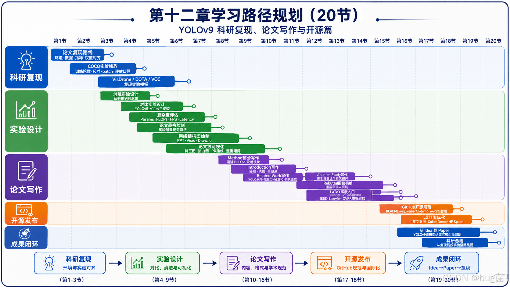
全文目录:
-
- 🔁 上期回顾
- 🎯 本节主题:Method 部分写作——如何描述 YOLOv9 改进模块
-
- 一、为什么 Method 是论文的灵魂
- 二、Method 部分的标准结构
- 三、YOLOv9 原始结构的写法——基线描述的艺术
-
- 3.1 基线描述的三个层次
- 3.2 YOLOv9 基线描述示例
- 四、核心改进模块的写法——这是 Method 的心脏
-
- 4.1 注意力机制改进——以在 YOLOv9 中加入 CBAM 为例
- 4.2 轻量化改进——以深度可分离卷积替换为例
- 4.3 多尺度特征融合改进——以 BiFPN 思路为例
- 五、损失函数写法——数学要漂亮,解释要到位
-
- 5.1 YOLOv9 原始损失函数的描述
- 5.2 改进损失函数的写法
- 六、完整 Method 写作流程——从零到一的实战演练
-
- 6.1 整体架构图(必须有)
- 6.2 完整 Method 英文写作示例
- 七、Python 代码实现与注释——让方法"活"起来
-
- 7.1 CBAM 模块实现
- 7.2 BiFPN 特征融合模块实现
- 7.3 将改进模块集成到 YOLOv9 的步骤说明
- 八、常见写作错误与修正——避开这些坑
-
- 8.1 错误一:只描述"做了什么",不说"为什么"
- 8.2 错误二:公式孤立,缺少变量说明
- 8.3 错误三:图文脱节
- 8.4 错误四:改进说明缺少"与基线的对比"
- 九、写完之后的自检清单
- 十、Method 写作的高阶技巧——让你的论文脱颖而出
-
- 10.1 "理论→实验"的呼应结构
- 10.2 用图说明"改进前后的对比"
- 10.3 定量说明改进的开销
- 十一、完整 Method 部分写作模板汇总
- 📅 下期预告:第11节——Introduction 写作:从痛点、挑战到贡献点
- 📌 附录
- 🧧🧧 文末福利,等你来拿!🧧🧧
- 🫵 Who am I?
写论文这件事,让我又爱又恨。爱的是每次把一个想法整理成文字、让别人能读懂的那一刻;恨的是Method部分——明明自己的模块做出来了,跑通了,指标也涨了,但就是不知道怎么"说清楚"。这节课我们就专门解决这个问题。
🔁 上期回顾
在上期《YOLOv9【第十二章:科研复现、论文写作与开源篇·第9节】特征图、热力图、PR 曲线、混淆矩阵论文级可视化!》内容中,我们系统讲解了特征图、热力图、PR 曲线与混淆矩阵的论文级可视化方法。回顾一下核心要点:
在那一节里,我们从"为什么要可视化"这个根本问题出发,厘清了一个重要认知:可视化不是装饰,而是证明。一张漂亮的 GradCAM 热力图,能直观说明你的模型"看"的位置更合理;一组对比 PR 曲线,能比单个 mAP 数字更有说服力地展示你在各个置信度阈值下的综合表现;而混淆矩阵则可以揭示你的模型在哪些类别上存在混淆,帮助审稿人和读者快速理解模型的局限性与改进方向。
具体工具层面,我们使用了 pytorch-grad-cam 实现 YOLOv9 特征热力图的提取,通过 matplotlib 绘制了符合论文审美标准的 PR 曲线组,并用 seaborn 对混淆矩阵做了规范化处理与颜色映射。每一个代码示例都附有详细注释,确保你不仅能"用",还能"懂"。
最重要的是,我们强调了图与文字配合的原则——可视化图像要在正文中有对应的文字描述,不能只放图不解释,审稿人不会替你分析。
好,带着这些积累,我们今天来啃最难的那块骨头:Method 部分写作。
🎯 本节主题:Method 部分写作——如何描述 YOLOv9 改进模块
一、为什么 Method 是论文的灵魂
很多同学在写论文的时候有一个误区:觉得 Introduction 最难写,因为要讲故事、讲动机。但实际上,真正决定一篇论文生死的,往往是 Method(方法)部分。
原因很简单:
Introduction 决定审稿人愿不愿意继续读,Method 决定他愿不愿意接受你。
Introduction 可以靠行文技巧和引用堆砌显得很扎实,但 Method 是硬货——你的改进模块到底是什么,它为什么有效,它和现有工作有什么本质区别,这些问题都必须在 Method 里回答清楚。写不清楚,或者写得含糊,审稿人就会质疑:这个模块到底有没有技术含量?作者自己理解吗?
另一个常见问题是:写 Method 时,作者自己懂,但读者读不懂。这是因为论文写作和技术实现是两种不同的认知模式。实现时你是从代码出发,一步步搭建;写作时你需要从原理出发,从动机到设计到实现再到效果,按照读者能接受的顺序来组织。
这就是今天这节课要解决的核心问题:如何把一个你亲手实现的改进模块,用清晰、规范、有说服力的学术语言描述出来。
二、Method 部分的标准结构
在正式动笔之前,我们先建立一个整体框架。一个规范的 Method 部分,通常包含以下几个层次:
#mermaid-svg-6Hd87TO80ez9WKUo{font-family:\”trebuchet ms\”,verdana,arial,sans-serif;font-size:16px;fill:#333;}@keyframes edge-animation-frame{from{stroke-dashoffset:0;}}@keyframes dash{to{stroke-dashoffset:0;}}#mermaid-svg-6Hd87TO80ez9WKUo .edge-animation-slow{stroke-dasharray:9,5!important;stroke-dashoffset:900;animation:dash 50s linear infinite;stroke-linecap:round;}#mermaid-svg-6Hd87TO80ez9WKUo .edge-animation-fast{stroke-dasharray:9,5!important;stroke-dashoffset:900;animation:dash 20s linear infinite;stroke-linecap:round;}#mermaid-svg-6Hd87TO80ez9WKUo .error-icon{fill:#552222;}#mermaid-svg-6Hd87TO80ez9WKUo .error-text{fill:#552222;stroke:#552222;}#mermaid-svg-6Hd87TO80ez9WKUo .edge-thickness-normal{stroke-width:1px;}#mermaid-svg-6Hd87TO80ez9WKUo .edge-thickness-thick{stroke-width:3.5px;}#mermaid-svg-6Hd87TO80ez9WKUo .edge-pattern-solid{stroke-dasharray:0;}#mermaid-svg-6Hd87TO80ez9WKUo .edge-thickness-invisible{stroke-width:0;fill:none;}#mermaid-svg-6Hd87TO80ez9WKUo .edge-pattern-dashed{stroke-dasharray:3;}#mermaid-svg-6Hd87TO80ez9WKUo .edge-pattern-dotted{stroke-dasharray:2;}#mermaid-svg-6Hd87TO80ez9WKUo .marker{fill:#333333;stroke:#333333;}#mermaid-svg-6Hd87TO80ez9WKUo .marker.cross{stroke:#333333;}#mermaid-svg-6Hd87TO80ez9WKUo svg{font-family:\”trebuchet ms\”,verdana,arial,sans-serif;font-size:16px;}#mermaid-svg-6Hd87TO80ez9WKUo p{margin:0;}#mermaid-svg-6Hd87TO80ez9WKUo .label{font-family:\”trebuchet ms\”,verdana,arial,sans-serif;color:#333;}#mermaid-svg-6Hd87TO80ez9WKUo .cluster-label text{fill:#333;}#mermaid-svg-6Hd87TO80ez9WKUo .cluster-label span{color:#333;}#mermaid-svg-6Hd87TO80ez9WKUo .cluster-label span p{background-color:transparent;}#mermaid-svg-6Hd87TO80ez9WKUo .label text,#mermaid-svg-6Hd87TO80ez9WKUo span{fill:#333;color:#333;}#mermaid-svg-6Hd87TO80ez9WKUo .node rect,#mermaid-svg-6Hd87TO80ez9WKUo .node circle,#mermaid-svg-6Hd87TO80ez9WKUo .node ellipse,#mermaid-svg-6Hd87TO80ez9WKUo .node polygon,#mermaid-svg-6Hd87TO80ez9WKUo .node path{fill:#ECECFF;stroke:#9370DB;stroke-width:1px;}#mermaid-svg-6Hd87TO80ez9WKUo .rough-node .label text,#mermaid-svg-6Hd87TO80ez9WKUo .node .label text,#mermaid-svg-6Hd87TO80ez9WKUo .image-shape .label,#mermaid-svg-6Hd87TO80ez9WKUo .icon-shape .label{text-anchor:middle;}#mermaid-svg-6Hd87TO80ez9WKUo .node .katex path{fill:#000;stroke:#000;stroke-width:1px;}#mermaid-svg-6Hd87TO80ez9WKUo .rough-node .label,#mermaid-svg-6Hd87TO80ez9WKUo .node .label,#mermaid-svg-6Hd87TO80ez9WKUo .image-shape .label,#mermaid-svg-6Hd87TO80ez9WKUo .icon-shape .label{text-align:center;}#mermaid-svg-6Hd87TO80ez9WKUo .node.clickable{cursor:pointer;}#mermaid-svg-6Hd87TO80ez9WKUo .root .anchor path{fill:#333333!important;stroke-width:0;stroke:#333333;}#mermaid-svg-6Hd87TO80ez9WKUo .arrowheadPath{fill:#333333;}#mermaid-svg-6Hd87TO80ez9WKUo .edgePath .path{stroke:#333333;stroke-width:2.0px;}#mermaid-svg-6Hd87TO80ez9WKUo .flowchart-link{stroke:#333333;fill:none;}#mermaid-svg-6Hd87TO80ez9WKUo .edgeLabel{background-color:rgba(232,232,232, 0.8);text-align:center;}#mermaid-svg-6Hd87TO80ez9WKUo .edgeLabel p{background-color:rgba(232,232,232, 0.8);}#mermaid-svg-6Hd87TO80ez9WKUo .edgeLabel rect{opacity:0.5;background-color:rgba(232,232,232, 0.8);fill:rgba(232,232,232, 0.8);}#mermaid-svg-6Hd87TO80ez9WKUo .labelBkg{background-color:rgba(232, 232, 232, 0.5);}#mermaid-svg-6Hd87TO80ez9WKUo .cluster rect{fill:#ffffde;stroke:#aaaa33;stroke-width:1px;}#mermaid-svg-6Hd87TO80ez9WKUo .cluster text{fill:#333;}#mermaid-svg-6Hd87TO80ez9WKUo .cluster span{color:#333;}#mermaid-svg-6Hd87TO80ez9WKUo div.mermaidTooltip{position:absolute;text-align:center;max-width:200px;padding:2px;font-family:\”trebuchet ms\”,verdana,arial,sans-serif;font-size:12px;background:hsl(80, 100%, 96.2745098039%);border:1px solid #aaaa33;border-radius:2px;pointer-events:none;z-index:100;}#mermaid-svg-6Hd87TO80ez9WKUo .flowchartTitleText{text-anchor:middle;font-size:18px;fill:#333;}#mermaid-svg-6Hd87TO80ez9WKUo rect.text{fill:none;stroke-width:0;}#mermaid-svg-6Hd87TO80ez9WKUo .icon-shape,#mermaid-svg-6Hd87TO80ez9WKUo .image-shape{background-color:rgba(232,232,232, 0.8);text-align:center;}#mermaid-svg-6Hd87TO80ez9WKUo .icon-shape p,#mermaid-svg-6Hd87TO80ez9WKUo .image-shape p{background-color:rgba(232,232,232, 0.8);padding:2px;}#mermaid-svg-6Hd87TO80ez9WKUo .icon-shape .label rect,#mermaid-svg-6Hd87TO80ez9WKUo .image-shape .label rect{opacity:0.5;background-color:rgba(232,232,232, 0.8);fill:rgba(232,232,232, 0.8);}#mermaid-svg-6Hd87TO80ez9WKUo .label-icon{display:inline-block;height:1em;overflow:visible;vertical-align:-0.125em;}#mermaid-svg-6Hd87TO80ez9WKUo .node .label-icon path{fill:currentColor;stroke:revert;stroke-width:revert;}#mermaid-svg-6Hd87TO80ez9WKUo :root{–mermaid-font-family:\”trebuchet ms\”,verdana,arial,sans-serif;}
Method 部分总览
2.1 Overall Architecture总体架构描述
2.2 改进模块详述Proposed Module
2.3 损失函数设计Loss Function
2.4 训练策略Training Strategy
描述基线模型 YOLOv9 的整体结构
指出改进位置与改进动机
理论动机Why this design?
结构细节How it works?
数学公式Formalization
与基线对比Difference from baseline
损失函数组成
各项权重说明
数据增强策略
优化器与学习率
其他超参数
这个框架不是死板的规定,不同的论文可以根据自己的改进点有所侧重。但核心逻辑是固定的:先讲整体,再讲局部;先讲为什么,再讲怎么做;先讲结构,再讲数学。
三、YOLOv9 原始结构的写法——基线描述的艺术
在讲自己的改进之前,你需要先描述基线模型。这一段看似简单,实则很有学问。
3.1 基线描述的三个层次
第一层:架构层面的描述
这一层告诉读者 YOLOv9 的宏观结构。注意不要陷入流水账式的罗列,而要突出对你的改进有意义的那些特性。
比如,如果你的改进是在 Neck 部分加入注意力机制,那你描述基线时就应该重点介绍 PAN 结构和特征融合机制,而不是花大量篇幅讲 Backbone 的细节。
第二层:关键机制的描述
YOLOv9 最核心的创新是 GELAN(Generalized Efficient Layer Aggregation Network) 和 PGI(Programmable Gradient Information)。如果你的改进与这两个机制有交互,就需要在这里讲清楚它们的原理。
第三层:局限性的引出
基线描述的最后,要自然地引出现有方法的局限性——也就是你改进的出发点。这是过渡到"改进模块"部分的关键桥梁。
3.2 YOLOv9 基线描述示例
以下是一段参考写法,展示如何用英文学术语言描述 YOLOv9 基线:
"YOLOv9 [cite] introduces two key innovations to address the information bottleneck problem in deep neural networks. The first is Programmable Gradient Information (PGI), which provides complete input information for the target task through reversible branches, ensuring reliable gradient information for network updates. The second is the Generalized Efficient Layer Aggregation Network (GELAN), which combines CSPNet and ELAN to achieve better parameter utilization efficiency.
However, despite these advances, YOLOv9 still exhibits limitations in [specific scenario, e.g., small object detection under complex backgrounds], primarily because [specific technical reason, e.g., the fixed receptive field size in the backbone limits the model’s ability to capture multi-scale contextual information]. This motivates our proposed [module name]."
注意几个细节:
- 引用 YOLOv9 的原始论文([cite]处填入你的参考文献编号)
- 用 “However” 自然转折,引出问题
- 问题描述要具体到技术层面,不能只说"性能不好"
四、核心改进模块的写法——这是 Method 的心脏
这部分是整个 Method 的重中之重。我会以几个常见的改进类型为例,分别讲解怎么写。
4.1 注意力机制改进——以在 YOLOv9 中加入 CBAM 为例
注意力机制是 YOLOv9 改进论文中最常见的方向之一。假设你在 YOLOv9 的 Neck 部分加入了 CBAM(Convolutional Block Attention Module),以下是完整的写作逻辑。
第一步:讲动机(Motivation)
不要上来就说"我加了一个CBAM"。先讲为什么要加。
“In object detection tasks, feature maps from different spatial locations and channels carry information of varying importance. Standard convolutional operations treat all spatial positions and channels equally, which may suppress discriminative features and amplify irrelevant background noise. To address this, we propose integrating a channel-spatial attention module into the feature pyramid network of YOLOv9, enabling the model to adaptively recalibrate feature responses both channel-wise and spatially.”
第二步:讲结构(Architecture)
这里要配合图示,用文字描述你的模块结构。
“As illustrated in Figure X, the proposed Attention-Enhanced Feature Pyramid (AEFP) module consists of three components: (1) a Channel Attention Module (CAM) that exploits the inter-channel relationship of features, (2) a Spatial Attention Module (SAM) that utilizes the inter-spatial relationship, and (3) a residual connection that preserves the original feature information to prevent gradient vanishing.”
第三步:讲数学(Formalization)
注意力机制一定要写数学公式,这是展示技术深度的关键。
对于 CBAM,标准的数学描述如下:
F
′
=
M
c
(
F
)
⊗
F
F' = M_c(F) \\otimes F
F′=Mc(F)⊗F
F
′
′
=
M
s
(
F
′
)
⊗
F
′
F'' = M_s(F') \\otimes F'
F′′=Ms(F′)⊗F′
其中:
-
F
∈
R
C
×
H
×
W
F \\in \\mathbb{R}^{C \\times H \\times W}
F∈RC×H×W 是输入特征图 -
M
c
(
F
)
∈
R
C
×
1
×
1
M_c(F) \\in \\mathbb{R}^{C \\times 1 \\times 1}
Mc(F)∈RC×1×1 是通道注意力图 -
M
s
(
F
′
)
∈
R
1
×
H
×
W
M_s(F') \\in \\mathbb{R}^{1 \\times H \\times W}
Ms(F′)∈R1×H×W 是空间注意力图 -
⊗
\\otimes
⊗ 表示逐元素相乘
通道注意力的计算:
M
c
(
F
)
=
σ
(
W
1
(
W
0
(
AvgPool
(
F
)
)
)
+
W
1
(
W
0
(
MaxPool
(
F
)
)
)
)
M_c(F) = \\sigma(W_1(W_0(\\text{AvgPool}(F))) + W_1(W_0(\\text{MaxPool}(F))))
Mc(F)=σ(W1(W0(AvgPool(F)))+W1(W0(MaxPool(F))))
空间注意力的计算:
M
s
(
F
′
)
=
σ
(
f
7
×
7
(
[
AvgPool
(
F
′
)
;
MaxPool
(
F
′
)
]
)
)
M_s(F') = \\sigma(f^{7\\times7}([\\text{AvgPool}(F'); \\text{MaxPool}(F')]))
Ms(F′)=σ(f7×7([AvgPool(F′);MaxPool(F′)]))
第四步:讲集成方式(Integration)
说清楚你把这个模块插在了 YOLOv9 的哪个位置,为什么选这个位置。
“We insert the AEFP module after each P3/P4/P5 feature fusion in the PAN neck of YOLOv9. This design choice is motivated by the observation that feature maps at the neck stage already contain rich semantic information from the backbone, making attention recalibration more effective compared to early-stage application.”
以下是对应的 Mermaid 结构图:
#mermaid-svg-kB6MFDL9m0Pldt1f{font-family:\”trebuchet ms\”,verdana,arial,sans-serif;font-size:16px;fill:#333;}@keyframes edge-animation-frame{from{stroke-dashoffset:0;}}@keyframes dash{to{stroke-dashoffset:0;}}#mermaid-svg-kB6MFDL9m0Pldt1f .edge-animation-slow{stroke-dasharray:9,5!important;stroke-dashoffset:900;animation:dash 50s linear infinite;stroke-linecap:round;}#mermaid-svg-kB6MFDL9m0Pldt1f .edge-animation-fast{stroke-dasharray:9,5!important;stroke-dashoffset:900;animation:dash 20s linear infinite;stroke-linecap:round;}#mermaid-svg-kB6MFDL9m0Pldt1f .error-icon{fill:#552222;}#mermaid-svg-kB6MFDL9m0Pldt1f .error-text{fill:#552222;stroke:#552222;}#mermaid-svg-kB6MFDL9m0Pldt1f .edge-thickness-normal{stroke-width:1px;}#mermaid-svg-kB6MFDL9m0Pldt1f .edge-thickness-thick{stroke-width:3.5px;}#mermaid-svg-kB6MFDL9m0Pldt1f .edge-pattern-solid{stroke-dasharray:0;}#mermaid-svg-kB6MFDL9m0Pldt1f .edge-thickness-invisible{stroke-width:0;fill:none;}#mermaid-svg-kB6MFDL9m0Pldt1f .edge-pattern-dashed{stroke-dasharray:3;}#mermaid-svg-kB6MFDL9m0Pldt1f .edge-pattern-dotted{stroke-dasharray:2;}#mermaid-svg-kB6MFDL9m0Pldt1f .marker{fill:#333333;stroke:#333333;}#mermaid-svg-kB6MFDL9m0Pldt1f .marker.cross{stroke:#333333;}#mermaid-svg-kB6MFDL9m0Pldt1f svg{font-family:\”trebuchet ms\”,verdana,arial,sans-serif;font-size:16px;}#mermaid-svg-kB6MFDL9m0Pldt1f p{margin:0;}#mermaid-svg-kB6MFDL9m0Pldt1f .label{font-family:\”trebuchet ms\”,verdana,arial,sans-serif;color:#333;}#mermaid-svg-kB6MFDL9m0Pldt1f .cluster-label text{fill:#333;}#mermaid-svg-kB6MFDL9m0Pldt1f .cluster-label span{color:#333;}#mermaid-svg-kB6MFDL9m0Pldt1f .cluster-label span p{background-color:transparent;}#mermaid-svg-kB6MFDL9m0Pldt1f .label text,#mermaid-svg-kB6MFDL9m0Pldt1f span{fill:#333;color:#333;}#mermaid-svg-kB6MFDL9m0Pldt1f .node rect,#mermaid-svg-kB6MFDL9m0Pldt1f .node circle,#mermaid-svg-kB6MFDL9m0Pldt1f .node ellipse,#mermaid-svg-kB6MFDL9m0Pldt1f .node polygon,#mermaid-svg-kB6MFDL9m0Pldt1f .node path{fill:#ECECFF;stroke:#9370DB;stroke-width:1px;}#mermaid-svg-kB6MFDL9m0Pldt1f .rough-node .label text,#mermaid-svg-kB6MFDL9m0Pldt1f .node .label text,#mermaid-svg-kB6MFDL9m0Pldt1f .image-shape .label,#mermaid-svg-kB6MFDL9m0Pldt1f .icon-shape .label{text-anchor:middle;}#mermaid-svg-kB6MFDL9m0Pldt1f .node .katex path{fill:#000;stroke:#000;stroke-width:1px;}#mermaid-svg-kB6MFDL9m0Pldt1f .rough-node .label,#mermaid-svg-kB6MFDL9m0Pldt1f .node .label,#mermaid-svg-kB6MFDL9m0Pldt1f .image-shape .label,#mermaid-svg-kB6MFDL9m0Pldt1f .icon-shape .label{text-align:center;}#mermaid-svg-kB6MFDL9m0Pldt1f .node.clickable{cursor:pointer;}#mermaid-svg-kB6MFDL9m0Pldt1f .root .anchor path{fill:#333333!important;stroke-width:0;stroke:#333333;}#mermaid-svg-kB6MFDL9m0Pldt1f .arrowheadPath{fill:#333333;}#mermaid-svg-kB6MFDL9m0Pldt1f .edgePath .path{stroke:#333333;stroke-width:2.0px;}#mermaid-svg-kB6MFDL9m0Pldt1f .flowchart-link{stroke:#333333;fill:none;}#mermaid-svg-kB6MFDL9m0Pldt1f .edgeLabel{background-color:rgba(232,232,232, 0.8);text-align:center;}#mermaid-svg-kB6MFDL9m0Pldt1f .edgeLabel p{background-color:rgba(232,232,232, 0.8);}#mermaid-svg-kB6MFDL9m0Pldt1f .edgeLabel rect{opacity:0.5;background-color:rgba(232,232,232, 0.8);fill:rgba(232,232,232, 0.8);}#mermaid-svg-kB6MFDL9m0Pldt1f .labelBkg{background-color:rgba(232, 232, 232, 0.5);}#mermaid-svg-kB6MFDL9m0Pldt1f .cluster rect{fill:#ffffde;stroke:#aaaa33;stroke-width:1px;}#mermaid-svg-kB6MFDL9m0Pldt1f .cluster text{fill:#333;}#mermaid-svg-kB6MFDL9m0Pldt1f .cluster span{color:#333;}#mermaid-svg-kB6MFDL9m0Pldt1f div.mermaidTooltip{position:absolute;text-align:center;max-width:200px;padding:2px;font-family:\”trebuchet ms\”,verdana,arial,sans-serif;font-size:12px;background:hsl(80, 100%, 96.2745098039%);border:1px solid #aaaa33;border-radius:2px;pointer-events:none;z-index:100;}#mermaid-svg-kB6MFDL9m0Pldt1f .flowchartTitleText{text-anchor:middle;font-size:18px;fill:#333;}#mermaid-svg-kB6MFDL9m0Pldt1f rect.text{fill:none;stroke-width:0;}#mermaid-svg-kB6MFDL9m0Pldt1f .icon-shape,#mermaid-svg-kB6MFDL9m0Pldt1f .image-shape{background-color:rgba(232,232,232, 0.8);text-align:center;}#mermaid-svg-kB6MFDL9m0Pldt1f .icon-shape p,#mermaid-svg-kB6MFDL9m0Pldt1f .image-shape p{background-color:rgba(232,232,232, 0.8);padding:2px;}#mermaid-svg-kB6MFDL9m0Pldt1f .icon-shape .label rect,#mermaid-svg-kB6MFDL9m0Pldt1f .image-shape .label rect{opacity:0.5;background-color:rgba(232,232,232, 0.8);fill:rgba(232,232,232, 0.8);}#mermaid-svg-kB6MFDL9m0Pldt1f .label-icon{display:inline-block;height:1em;overflow:visible;vertical-align:-0.125em;}#mermaid-svg-kB6MFDL9m0Pldt1f .node .label-icon path{fill:currentColor;stroke:revert;stroke-width:revert;}#mermaid-svg-kB6MFDL9m0Pldt1f :root{–mermaid-font-family:\”trebuchet ms\”,verdana,arial,sans-serif;}
改进的 PAN Neck
YOLOv9 Backbone (GELAN)
检测头
Multi-scaleDetection
AEFP 模块内部
输入特征 FC×H×W
Channel AttentionMc(F)
Spatial AttentionMs(F')
输出特征 F''C×H×W
残差连接
C3 特征P3: 80×80
C4 特征P4: 40×40
C5 特征P5: 20×20
AEFP Module@P5
AEFP Module@P4
AEFP Module@P3
特征融合Feature Fusion
4.2 轻量化改进——以深度可分离卷积替换为例
如果你的改进方向是模型轻量化,写作逻辑会有所不同。轻量化改进的 Method 写作需要强调效率与精度的权衡,并且要用数据说话。
动机写法:
“While YOLOv9 achieves state-of-the-art detection performance, its deployment on resource-constrained edge devices remains challenging due to high computational complexity. The standard 3×3 convolutions in GELAN blocks account for approximately 73% of total FLOPs, motivating us to explore more efficient alternatives.”
结构描述:
在描述深度可分离卷积时,一定要把标准卷积和深度可分离卷积的计算量对比用公式写出来,这是最有说服力的地方。
标准卷积的计算量:
FLOPs
∗
std
=
2
×
H
×
W
×
C
∗
i
n
×
C
o
u
t
×
K
2
\\text{FLOPs}*{\\text{std}} = 2 \\times H \\times W \\times C*{in} \\times C_{out} \\times K^2
FLOPs∗std=2×H×W×C∗in×Cout×K2
深度可分离卷积的计算量:
FLOPs
∗
dw
=
2
×
H
×
W
×
C
∗
i
n
×
K
2
+
2
×
H
×
W
×
C
i
n
×
C
o
u
t
\\text{FLOPs}*{\\text{dw}} = 2 \\times H \\times W \\times C*{in} \\times K^2 + 2 \\times H \\times W \\times C_{in} \\times C_{out}
FLOPs∗dw=2×H×W×C∗in×K2+2×H×W×Cin×Cout
压缩比:
Ratio
=
FLOPs
∗
dw
FLOPs
∗
std
=
1
C
o
u
t
+
1
K
2
\\text{Ratio} = \\frac{\\text{FLOPs}*{\\text{dw}}}{\\text{FLOPs}*{\\text{std}}} = \\frac{1}{C_{out}} + \\frac{1}{K^2}
Ratio=FLOPs∗stdFLOPs∗dw=Cout1+K21
当
K
=
3
,
C
o
u
t
=
256
K=3, C_{out}=256
K=3,Cout=256 时,压缩比约为
1
9
\\frac{1}{9}
91,即理论上可以减少约 88.9% 的计算量。
#mermaid-svg-qjf26vqj0Cz1FuDl{font-family:\”trebuchet ms\”,verdana,arial,sans-serif;font-size:16px;fill:#333;}@keyframes edge-animation-frame{from{stroke-dashoffset:0;}}@keyframes dash{to{stroke-dashoffset:0;}}#mermaid-svg-qjf26vqj0Cz1FuDl .edge-animation-slow{stroke-dasharray:9,5!important;stroke-dashoffset:900;animation:dash 50s linear infinite;stroke-linecap:round;}#mermaid-svg-qjf26vqj0Cz1FuDl .edge-animation-fast{stroke-dasharray:9,5!important;stroke-dashoffset:900;animation:dash 20s linear infinite;stroke-linecap:round;}#mermaid-svg-qjf26vqj0Cz1FuDl .error-icon{fill:#552222;}#mermaid-svg-qjf26vqj0Cz1FuDl .error-text{fill:#552222;stroke:#552222;}#mermaid-svg-qjf26vqj0Cz1FuDl .edge-thickness-normal{stroke-width:1px;}#mermaid-svg-qjf26vqj0Cz1FuDl .edge-thickness-thick{stroke-width:3.5px;}#mermaid-svg-qjf26vqj0Cz1FuDl .edge-pattern-solid{stroke-dasharray:0;}#mermaid-svg-qjf26vqj0Cz1FuDl .edge-thickness-invisible{stroke-width:0;fill:none;}#mermaid-svg-qjf26vqj0Cz1FuDl .edge-pattern-dashed{stroke-dasharray:3;}#mermaid-svg-qjf26vqj0Cz1FuDl .edge-pattern-dotted{stroke-dasharray:2;}#mermaid-svg-qjf26vqj0Cz1FuDl .marker{fill:#333333;stroke:#333333;}#mermaid-svg-qjf26vqj0Cz1FuDl .marker.cross{stroke:#333333;}#mermaid-svg-qjf26vqj0Cz1FuDl svg{font-family:\”trebuchet ms\”,verdana,arial,sans-serif;font-size:16px;}#mermaid-svg-qjf26vqj0Cz1FuDl p{margin:0;}#mermaid-svg-qjf26vqj0Cz1FuDl .label{font-family:\”trebuchet ms\”,verdana,arial,sans-serif;color:#333;}#mermaid-svg-qjf26vqj0Cz1FuDl .cluster-label text{fill:#333;}#mermaid-svg-qjf26vqj0Cz1FuDl .cluster-label span{color:#333;}#mermaid-svg-qjf26vqj0Cz1FuDl .cluster-label span p{background-color:transparent;}#mermaid-svg-qjf26vqj0Cz1FuDl .label text,#mermaid-svg-qjf26vqj0Cz1FuDl span{fill:#333;color:#333;}#mermaid-svg-qjf26vqj0Cz1FuDl .node rect,#mermaid-svg-qjf26vqj0Cz1FuDl .node circle,#mermaid-svg-qjf26vqj0Cz1FuDl .node ellipse,#mermaid-svg-qjf26vqj0Cz1FuDl .node polygon,#mermaid-svg-qjf26vqj0Cz1FuDl .node path{fill:#ECECFF;stroke:#9370DB;stroke-width:1px;}#mermaid-svg-qjf26vqj0Cz1FuDl .rough-node .label text,#mermaid-svg-qjf26vqj0Cz1FuDl .node .label text,#mermaid-svg-qjf26vqj0Cz1FuDl .image-shape .label,#mermaid-svg-qjf26vqj0Cz1FuDl .icon-shape .label{text-anchor:middle;}#mermaid-svg-qjf26vqj0Cz1FuDl .node .katex path{fill:#000;stroke:#000;stroke-width:1px;}#mermaid-svg-qjf26vqj0Cz1FuDl .rough-node .label,#mermaid-svg-qjf26vqj0Cz1FuDl .node .label,#mermaid-svg-qjf26vqj0Cz1FuDl .image-shape .label,#mermaid-svg-qjf26vqj0Cz1FuDl .icon-shape .label{text-align:center;}#mermaid-svg-qjf26vqj0Cz1FuDl .node.clickable{cursor:pointer;}#mermaid-svg-qjf26vqj0Cz1FuDl .root .anchor path{fill:#333333!important;stroke-width:0;stroke:#333333;}#mermaid-svg-qjf26vqj0Cz1FuDl .arrowheadPath{fill:#333333;}#mermaid-svg-qjf26vqj0Cz1FuDl .edgePath .path{stroke:#333333;stroke-width:2.0px;}#mermaid-svg-qjf26vqj0Cz1FuDl .flowchart-link{stroke:#333333;fill:none;}#mermaid-svg-qjf26vqj0Cz1FuDl .edgeLabel{background-color:rgba(232,232,232, 0.8);text-align:center;}#mermaid-svg-qjf26vqj0Cz1FuDl .edgeLabel p{background-color:rgba(232,232,232, 0.8);}#mermaid-svg-qjf26vqj0Cz1FuDl .edgeLabel rect{opacity:0.5;background-color:rgba(232,232,232, 0.8);fill:rgba(232,232,232, 0.8);}#mermaid-svg-qjf26vqj0Cz1FuDl .labelBkg{background-color:rgba(232, 232, 232, 0.5);}#mermaid-svg-qjf26vqj0Cz1FuDl .cluster rect{fill:#ffffde;stroke:#aaaa33;stroke-width:1px;}#mermaid-svg-qjf26vqj0Cz1FuDl .cluster text{fill:#333;}#mermaid-svg-qjf26vqj0Cz1FuDl .cluster span{color:#333;}#mermaid-svg-qjf26vqj0Cz1FuDl div.mermaidTooltip{position:absolute;text-align:center;max-width:200px;padding:2px;font-family:\”trebuchet ms\”,verdana,arial,sans-serif;font-size:12px;background:hsl(80, 100%, 96.2745098039%);border:1px solid #aaaa33;border-radius:2px;pointer-events:none;z-index:100;}#mermaid-svg-qjf26vqj0Cz1FuDl .flowchartTitleText{text-anchor:middle;font-size:18px;fill:#333;}#mermaid-svg-qjf26vqj0Cz1FuDl rect.text{fill:none;stroke-width:0;}#mermaid-svg-qjf26vqj0Cz1FuDl .icon-shape,#mermaid-svg-qjf26vqj0Cz1FuDl .image-shape{background-color:rgba(232,232,232, 0.8);text-align:center;}#mermaid-svg-qjf26vqj0Cz1FuDl .icon-shape p,#mermaid-svg-qjf26vqj0Cz1FuDl .image-shape p{background-color:rgba(232,232,232, 0.8);padding:2px;}#mermaid-svg-qjf26vqj0Cz1FuDl .icon-shape .label rect,#mermaid-svg-qjf26vqj0Cz1FuDl .image-shape .label rect{opacity:0.5;background-color:rgba(232,232,232, 0.8);fill:rgba(232,232,232, 0.8);}#mermaid-svg-qjf26vqj0Cz1FuDl .label-icon{display:inline-block;height:1em;overflow:visible;vertical-align:-0.125em;}#mermaid-svg-qjf26vqj0Cz1FuDl .node .label-icon path{fill:currentColor;stroke:revert;stroke-width:revert;}#mermaid-svg-qjf26vqj0Cz1FuDl :root{–mermaid-font-family:\”trebuchet ms\”,verdana,arial,sans-serif;}
替换为
深度可分离卷积 Depthwise Separable Conv
输入C_in×H×W
Depthwise Conv3×3, C_in→C_in
Pointwise Conv1×1, C_in→C_out
输出C_out×H×W
FLOPs ≈ FLOPs_std / 9
标准卷积 Standard Conv
输入C_in×H×W
3×3 ConvC_in→C_out
输出C_out×H×W
FLOPs: 2×H×W×C_in×C_out×9
4.3 多尺度特征融合改进——以 BiFPN 思路为例
这类改进涉及到特征金字塔的结构变化,写法上需要清晰地描述信息流动路径。
动机写法:
“The standard PAN neck in YOLOv9 employs a simple top-down and bottom-up feature fusion strategy, where all input features are treated with equal contribution weights. This uniform weighting may be suboptimal because input features at different resolutions carry semantically different information. For instance, high-resolution features contain rich spatial details while low-resolution features encode stronger semantic context.”
结构描述:
BiFPN 的核心是可学习的特征融合权重,数学表达如下:
O
=
∑
i
w
i
ϵ
+
∑
j
w
j
⋅
I
i
O = \\sum_{i} \\frac{w_i}{\\epsilon + \\sum_j w_j} \\cdot I_i
O=i∑ϵ+∑jwjwi⋅Ii
其中
w
i
>
0
w_i > 0
wi>0 通过 ReLU 函数保证,
ϵ
=
0.0001
\\epsilon = 0.0001
ϵ=0.0001 防止数值不稳定。
#mermaid-svg-O7hcE0sXPvYNETQA{font-family:\”trebuchet ms\”,verdana,arial,sans-serif;font-size:16px;fill:#333;}@keyframes edge-animation-frame{from{stroke-dashoffset:0;}}@keyframes dash{to{stroke-dashoffset:0;}}#mermaid-svg-O7hcE0sXPvYNETQA .edge-animation-slow{stroke-dasharray:9,5!important;stroke-dashoffset:900;animation:dash 50s linear infinite;stroke-linecap:round;}#mermaid-svg-O7hcE0sXPvYNETQA .edge-animation-fast{stroke-dasharray:9,5!important;stroke-dashoffset:900;animation:dash 20s linear infinite;stroke-linecap:round;}#mermaid-svg-O7hcE0sXPvYNETQA .error-icon{fill:#552222;}#mermaid-svg-O7hcE0sXPvYNETQA .error-text{fill:#552222;stroke:#552222;}#mermaid-svg-O7hcE0sXPvYNETQA .edge-thickness-normal{stroke-width:1px;}#mermaid-svg-O7hcE0sXPvYNETQA .edge-thickness-thick{stroke-width:3.5px;}#mermaid-svg-O7hcE0sXPvYNETQA .edge-pattern-solid{stroke-dasharray:0;}#mermaid-svg-O7hcE0sXPvYNETQA .edge-thickness-invisible{stroke-width:0;fill:none;}#mermaid-svg-O7hcE0sXPvYNETQA .edge-pattern-dashed{stroke-dasharray:3;}#mermaid-svg-O7hcE0sXPvYNETQA .edge-pattern-dotted{stroke-dasharray:2;}#mermaid-svg-O7hcE0sXPvYNETQA .marker{fill:#333333;stroke:#333333;}#mermaid-svg-O7hcE0sXPvYNETQA .marker.cross{stroke:#333333;}#mermaid-svg-O7hcE0sXPvYNETQA svg{font-family:\”trebuchet ms\”,verdana,arial,sans-serif;font-size:16px;}#mermaid-svg-O7hcE0sXPvYNETQA p{margin:0;}#mermaid-svg-O7hcE0sXPvYNETQA .label{font-family:\”trebuchet ms\”,verdana,arial,sans-serif;color:#333;}#mermaid-svg-O7hcE0sXPvYNETQA .cluster-label text{fill:#333;}#mermaid-svg-O7hcE0sXPvYNETQA .cluster-label span{color:#333;}#mermaid-svg-O7hcE0sXPvYNETQA .cluster-label span p{background-color:transparent;}#mermaid-svg-O7hcE0sXPvYNETQA .label text,#mermaid-svg-O7hcE0sXPvYNETQA span{fill:#333;color:#333;}#mermaid-svg-O7hcE0sXPvYNETQA .node rect,#mermaid-svg-O7hcE0sXPvYNETQA .node circle,#mermaid-svg-O7hcE0sXPvYNETQA .node ellipse,#mermaid-svg-O7hcE0sXPvYNETQA .node polygon,#mermaid-svg-O7hcE0sXPvYNETQA .node path{fill:#ECECFF;stroke:#9370DB;stroke-width:1px;}#mermaid-svg-O7hcE0sXPvYNETQA .rough-node .label text,#mermaid-svg-O7hcE0sXPvYNETQA .node .label text,#mermaid-svg-O7hcE0sXPvYNETQA .image-shape .label,#mermaid-svg-O7hcE0sXPvYNETQA .icon-shape .label{text-anchor:middle;}#mermaid-svg-O7hcE0sXPvYNETQA .node .katex path{fill:#000;stroke:#000;stroke-width:1px;}#mermaid-svg-O7hcE0sXPvYNETQA .rough-node .label,#mermaid-svg-O7hcE0sXPvYNETQA .node .label,#mermaid-svg-O7hcE0sXPvYNETQA .image-shape .label,#mermaid-svg-O7hcE0sXPvYNETQA .icon-shape .label{text-align:center;}#mermaid-svg-O7hcE0sXPvYNETQA .node.clickable{cursor:pointer;}#mermaid-svg-O7hcE0sXPvYNETQA .root .anchor path{fill:#333333!important;stroke-width:0;stroke:#333333;}#mermaid-svg-O7hcE0sXPvYNETQA .arrowheadPath{fill:#333333;}#mermaid-svg-O7hcE0sXPvYNETQA .edgePath .path{stroke:#333333;stroke-width:2.0px;}#mermaid-svg-O7hcE0sXPvYNETQA .flowchart-link{stroke:#333333;fill:none;}#mermaid-svg-O7hcE0sXPvYNETQA .edgeLabel{background-color:rgba(232,232,232, 0.8);text-align:center;}#mermaid-svg-O7hcE0sXPvYNETQA .edgeLabel p{background-color:rgba(232,232,232, 0.8);}#mermaid-svg-O7hcE0sXPvYNETQA .edgeLabel rect{opacity:0.5;background-color:rgba(232,232,232, 0.8);fill:rgba(232,232,232, 0.8);}#mermaid-svg-O7hcE0sXPvYNETQA .labelBkg{background-color:rgba(232, 232, 232, 0.5);}#mermaid-svg-O7hcE0sXPvYNETQA .cluster rect{fill:#ffffde;stroke:#aaaa33;stroke-width:1px;}#mermaid-svg-O7hcE0sXPvYNETQA .cluster text{fill:#333;}#mermaid-svg-O7hcE0sXPvYNETQA .cluster span{color:#333;}#mermaid-svg-O7hcE0sXPvYNETQA div.mermaidTooltip{position:absolute;text-align:center;max-width:200px;padding:2px;font-family:\”trebuchet ms\”,verdana,arial,sans-serif;font-size:12px;background:hsl(80, 100%, 96.2745098039%);border:1px solid #aaaa33;border-radius:2px;pointer-events:none;z-index:100;}#mermaid-svg-O7hcE0sXPvYNETQA .flowchartTitleText{text-anchor:middle;font-size:18px;fill:#333;}#mermaid-svg-O7hcE0sXPvYNETQA rect.text{fill:none;stroke-width:0;}#mermaid-svg-O7hcE0sXPvYNETQA .icon-shape,#mermaid-svg-O7hcE0sXPvYNETQA .image-shape{background-color:rgba(232,232,232, 0.8);text-align:center;}#mermaid-svg-O7hcE0sXPvYNETQA .icon-shape p,#mermaid-svg-O7hcE0sXPvYNETQA .image-shape p{background-color:rgba(232,232,232, 0.8);padding:2px;}#mermaid-svg-O7hcE0sXPvYNETQA .icon-shape .label rect,#mermaid-svg-O7hcE0sXPvYNETQA .image-shape .label rect{opacity:0.5;background-color:rgba(232,232,232, 0.8);fill:rgba(232,232,232, 0.8);}#mermaid-svg-O7hcE0sXPvYNETQA .label-icon{display:inline-block;height:1em;overflow:visible;vertical-align:-0.125em;}#mermaid-svg-O7hcE0sXPvYNETQA .node .label-icon path{fill:currentColor;stroke:revert;stroke-width:revert;}#mermaid-svg-O7hcE0sXPvYNETQA :root{–mermaid-font-family:\”trebuchet ms\”,verdana,arial,sans-serif;}
改进为
改进 BiFPN Neck
w1
w2
skip
w3
w4
w5
w6
w7
w8
P5
加权融合@P4
P4
P3
加权融合@P3
加权融合@P4 Bottom-up
加权融合@P5 Bottom-up
原始 PAN Neck
Top-down
Top-down
Bottom-up
Bottom-up
P520×20
P440×40
P380×80
P4'40×40
P5'20×20
五、损失函数写法——数学要漂亮,解释要到位
损失函数部分是 Method 中另一个技术难点。很多同学只是把公式粘贴上去,但不解释各项的物理意义,这会让审稿人觉得你不理解自己在做什么。
5.1 YOLOv9 原始损失函数的描述
YOLOv9 的总损失函数由三部分组成:
L
=
λ
1
L
∗
b
o
x
+
λ
2
L
∗
c
l
s
+
λ
3
L
d
f
l
\\mathcal{L} = \\lambda_1 \\mathcal{L}*{box} + \\lambda_2 \\mathcal{L}*{cls} + \\lambda_3 \\mathcal{L}_{dfl}
L=λ1L∗box+λ2L∗cls+λ3Ldfl
其中:
-
L
b
o
x
\\mathcal{L}_{box}
Lbox:边界框回归损失(CIoU Loss) -
L
c
l
s
\\mathcal{L}_{cls}
Lcls:分类损失(Binary Cross-Entropy with Sigmoid) -
L
d
f
l
\\mathcal{L}_{dfl}
Ldfl:分布焦点损失(Distribution Focal Loss)
描述这部分时,要解释每一项为什么存在,而不只是写公式。
CIoU Loss 的描述示例:
"The bounding box regression loss
L
b
o
x
\\mathcal{L}_{box}
Lbox is computed using Complete Intersection over Union (CIoU) loss, which simultaneously considers overlap area, center distance, and aspect ratio consistency:
L
C
I
o
U
=
1
−
I
o
U
+
ρ
2
(
b
,
b
g
t
)
c
2
+
α
v
\\mathcal{L}_{CIoU} = 1 – IoU + \\frac{\\rho^2(b, b^{gt})}{c^2} + \\alpha v
LCIoU=1−IoU+c2ρ2(b,bgt)+αv
where
ρ
(
⋅
)
\\rho(\\cdot)
ρ(⋅) denotes the Euclidean distance,
c
c
c is the diagonal length of the smallest enclosing box,
v
v
v measures aspect ratio consistency, and
α
\\alpha
α is a trade-off parameter. This formulation provides more complete geometric alignment signals compared to vanilla IoU loss."
5.2 改进损失函数的写法
如果你改动了损失函数(例如引入 Focal Loss 或 WIoU),写作时要遵循以下结构:
以引入 Wise-IoU(WIoU)为例:
"Standard IoU-based losses assign equal optimization focus to all samples regardless of their geometric quality. To address this, we adopt Wise-IoU [cite], which introduces a dynamic focusing coefficient
β
\\beta
β to down-weight the loss contribution from samples with excessively large geometric deviations:
L
∗
W
I
o
U
=
r
⋅
L
∗
I
o
U
\\mathcal{L}*{WIoU} = r \\cdot \\mathcal{L}*{IoU}
L∗WIoU=r⋅L∗IoU
where
r
=
e
(
IoU
∗
n
o
r
m
)
e
∈
[
1
e
,
1
]
r = \\frac{e^{(\\text{IoU}*{norm})}}{e} \\in [\\frac{1}{e}, 1]
r=ee(IoU∗norm)∈[e1,1] is the focusing factor, and
IoU
∗
n
o
r
m
\\text{IoU}*{norm}
IoU∗norm is the normalized IoU value. This design effectively reduces the influence of geometric outliers during training while maintaining stable optimization for high-quality anchor-target pairs."
六、完整 Method 写作流程——从零到一的实战演练
光说原理不过瘾,我们来做一个完整的实战演练。假设你的论文题目是:
“YOLOv9-CBAM-BiFPN: Enhancing Small Object Detection via Attention-Guided Multi-Scale Feature Fusion”
下面我展示完整的 Method 部分写作流程,包括中文思路分析和英文示例。
6.1 整体架构图(必须有)
任何一篇检测算法论文,Method 里第一个图必须是你的整体架构图。
#mermaid-svg-0f4UssuzFdBIgljm{font-family:\”trebuchet ms\”,verdana,arial,sans-serif;font-size:16px;fill:#333;}@keyframes edge-animation-frame{from{stroke-dashoffset:0;}}@keyframes dash{to{stroke-dashoffset:0;}}#mermaid-svg-0f4UssuzFdBIgljm .edge-animation-slow{stroke-dasharray:9,5!important;stroke-dashoffset:900;animation:dash 50s linear infinite;stroke-linecap:round;}#mermaid-svg-0f4UssuzFdBIgljm .edge-animation-fast{stroke-dasharray:9,5!important;stroke-dashoffset:900;animation:dash 20s linear infinite;stroke-linecap:round;}#mermaid-svg-0f4UssuzFdBIgljm .error-icon{fill:#552222;}#mermaid-svg-0f4UssuzFdBIgljm .error-text{fill:#552222;stroke:#552222;}#mermaid-svg-0f4UssuzFdBIgljm .edge-thickness-normal{stroke-width:1px;}#mermaid-svg-0f4UssuzFdBIgljm .edge-thickness-thick{stroke-width:3.5px;}#mermaid-svg-0f4UssuzFdBIgljm .edge-pattern-solid{stroke-dasharray:0;}#mermaid-svg-0f4UssuzFdBIgljm .edge-thickness-invisible{stroke-width:0;fill:none;}#mermaid-svg-0f4UssuzFdBIgljm .edge-pattern-dashed{stroke-dasharray:3;}#mermaid-svg-0f4UssuzFdBIgljm .edge-pattern-dotted{stroke-dasharray:2;}#mermaid-svg-0f4UssuzFdBIgljm .marker{fill:#333333;stroke:#333333;}#mermaid-svg-0f4UssuzFdBIgljm .marker.cross{stroke:#333333;}#mermaid-svg-0f4UssuzFdBIgljm svg{font-family:\”trebuchet ms\”,verdana,arial,sans-serif;font-size:16px;}#mermaid-svg-0f4UssuzFdBIgljm p{margin:0;}#mermaid-svg-0f4UssuzFdBIgljm .label{font-family:\”trebuchet ms\”,verdana,arial,sans-serif;color:#333;}#mermaid-svg-0f4UssuzFdBIgljm .cluster-label text{fill:#333;}#mermaid-svg-0f4UssuzFdBIgljm .cluster-label span{color:#333;}#mermaid-svg-0f4UssuzFdBIgljm .cluster-label span p{background-color:transparent;}#mermaid-svg-0f4UssuzFdBIgljm .label text,#mermaid-svg-0f4UssuzFdBIgljm span{fill:#333;color:#333;}#mermaid-svg-0f4UssuzFdBIgljm .node rect,#mermaid-svg-0f4UssuzFdBIgljm .node circle,#mermaid-svg-0f4UssuzFdBIgljm .node ellipse,#mermaid-svg-0f4UssuzFdBIgljm .node polygon,#mermaid-svg-0f4UssuzFdBIgljm .node path{fill:#ECECFF;stroke:#9370DB;stroke-width:1px;}#mermaid-svg-0f4UssuzFdBIgljm .rough-node .label text,#mermaid-svg-0f4UssuzFdBIgljm .node .label text,#mermaid-svg-0f4UssuzFdBIgljm .image-shape .label,#mermaid-svg-0f4UssuzFdBIgljm .icon-shape .label{text-anchor:middle;}#mermaid-svg-0f4UssuzFdBIgljm .node .katex path{fill:#000;stroke:#000;stroke-width:1px;}#mermaid-svg-0f4UssuzFdBIgljm .rough-node .label,#mermaid-svg-0f4UssuzFdBIgljm .node .label,#mermaid-svg-0f4UssuzFdBIgljm .image-shape .label,#mermaid-svg-0f4UssuzFdBIgljm .icon-shape .label{text-align:center;}#mermaid-svg-0f4UssuzFdBIgljm .node.clickable{cursor:pointer;}#mermaid-svg-0f4UssuzFdBIgljm .root .anchor path{fill:#333333!important;stroke-width:0;stroke:#333333;}#mermaid-svg-0f4UssuzFdBIgljm .arrowheadPath{fill:#333333;}#mermaid-svg-0f4UssuzFdBIgljm .edgePath .path{stroke:#333333;stroke-width:2.0px;}#mermaid-svg-0f4UssuzFdBIgljm .flowchart-link{stroke:#333333;fill:none;}#mermaid-svg-0f4UssuzFdBIgljm .edgeLabel{background-color:rgba(232,232,232, 0.8);text-align:center;}#mermaid-svg-0f4UssuzFdBIgljm .edgeLabel p{background-color:rgba(232,232,232, 0.8);}#mermaid-svg-0f4UssuzFdBIgljm .edgeLabel rect{opacity:0.5;background-color:rgba(232,232,232, 0.8);fill:rgba(232,232,232, 0.8);}#mermaid-svg-0f4UssuzFdBIgljm .labelBkg{background-color:rgba(232, 232, 232, 0.5);}#mermaid-svg-0f4UssuzFdBIgljm .cluster rect{fill:#ffffde;stroke:#aaaa33;stroke-width:1px;}#mermaid-svg-0f4UssuzFdBIgljm .cluster text{fill:#333;}#mermaid-svg-0f4UssuzFdBIgljm .cluster span{color:#333;}#mermaid-svg-0f4UssuzFdBIgljm div.mermaidTooltip{position:absolute;text-align:center;max-width:200px;padding:2px;font-family:\”trebuchet ms\”,verdana,arial,sans-serif;font-size:12px;background:hsl(80, 100%, 96.2745098039%);border:1px solid #aaaa33;border-radius:2px;pointer-events:none;z-index:100;}#mermaid-svg-0f4UssuzFdBIgljm .flowchartTitleText{text-anchor:middle;font-size:18px;fill:#333;}#mermaid-svg-0f4UssuzFdBIgljm rect.text{fill:none;stroke-width:0;}#mermaid-svg-0f4UssuzFdBIgljm .icon-shape,#mermaid-svg-0f4UssuzFdBIgljm .image-shape{background-color:rgba(232,232,232, 0.8);text-align:center;}#mermaid-svg-0f4UssuzFdBIgljm .icon-shape p,#mermaid-svg-0f4UssuzFdBIgljm .image-shape p{background-color:rgba(232,232,232, 0.8);padding:2px;}#mermaid-svg-0f4UssuzFdBIgljm .icon-shape .label rect,#mermaid-svg-0f4UssuzFdBIgljm .image-shape .label rect{opacity:0.5;background-color:rgba(232,232,232, 0.8);fill:rgba(232,232,232, 0.8);}#mermaid-svg-0f4UssuzFdBIgljm .label-icon{display:inline-block;height:1em;overflow:visible;vertical-align:-0.125em;}#mermaid-svg-0f4UssuzFdBIgljm .node .label-icon path{fill:currentColor;stroke:revert;stroke-width:revert;}#mermaid-svg-0f4UssuzFdBIgljm :root{–mermaid-font-family:\”trebuchet ms\”,verdana,arial,sans-serif;}
检测头 Detection Head
改进的 BiFPN + CBAM Neck
GELAN Backbone(YOLOv9 原始)
梯度辅助
PGI 辅助训练分支(YOLOv9 原始)
Auxiliary Branch
输入
Input Image640×640×3
Stem Layer
GELAN Block ×3320×320
GELAN Block ×6160×160
GELAN Block ×980×80 → P3
GELAN Block ×340×40 → P4
GELAN Block ×320×20 → P5
BiFPN 双向特征融合
CBAM @ P380×80
CBAM @ P440×40
CBAM @ P520×20
Large Obj20×20
Medium Obj40×40
Small Obj80×80
6.2 完整 Method 英文写作示例
以下是一段完整的 Method 部分示例,大约 600 词,供你参考或修改使用:
3. Methodology
3.1 Overall Architecture
As illustrated in Figure 1, the proposed YOLOv9-CBAM-BiFPN builds upon the YOLOv9 framework while introducing two targeted modifications to the neck architecture. The backbone retains the original GELAN structure, which employs gradient path planning through Programmable Gradient Information (PGI) to ensure complete information flow during training. The primary modifications are: (1) replacing the standard PAN neck with a Bidirectional Feature Pyramid Network (BiFPN) for more effective multi-scale feature fusion, and (2) embedding Convolutional Block Attention Modules (CBAM) at each feature pyramid level to adaptively recalibrate feature responses.
The design rationale is twofold. First, small objects in complex scenes often produce weak activation responses that are easily overwhelmed by background features during fusion. Second, standard equal-weight feature aggregation fails to distinguish the varying semantic richness of features at different resolution scales. Our modifications directly address these two issues.
3.2 Attention-Enhanced Bidirectional Feature Fusion
3.2.1 BiFPN Neck
The standard PAN neck in YOLOv9 fuses multi-scale features through a top-down followed by bottom-up pathway, treating all input features with equal contribution. We replace this with BiFPN [cite], which introduces learnable scalar weights for each feature input during fusion:
P
~
∗
l
o
u
t
=
∑
∗
i
w
i
ϵ
+
∑
j
w
j
⋅
P
l
i
n
,
i
,
w
i
=
ReLU
(
w
i
0
)
\\tilde{P}*l^{out} = \\sum*{i} \\frac{w_i}{\\epsilon + \\sum_j w_j} \\cdot P_l^{in,i}, \\quad w_i = \\text{ReLU}(w_i^0)
P~∗lout=∑∗iϵ+∑jwjwi⋅Plin,i,wi=ReLU(wi0)
where
P
l
i
n
,
i
P_l^{in,i}
Plin,i denotes the
i
i
i-th input feature at pyramid level
l
l
l,
w
i
w_i
wi are learnable weights constrained to be non-negative via ReLU, and
ϵ
=
10
−
4
\\epsilon = 10^{-4}
ϵ=10−4 ensures numerical stability. This formulation enables the model to learn optimal fusion ratios automatically, prioritizing semantically richer features at each scale.
3.2.2 CBAM Integration
Following each BiFPN fusion node, we apply CBAM to refine the fused feature map
F
f
u
s
e
d
F_{fused}
Ffused. The attention computation proceeds sequentially through channel and spatial dimensions:
F
′
=
M
∗
c
(
F
∗
f
u
s
e
d
)
⊙
F
f
u
s
e
d
F' = \\mathcal{M}*c(F*{fused}) \\odot F_{fused}
F′=M∗c(F∗fused)⊙Ffused
F
′
′
=
M
s
(
F
′
)
⊙
F
′
F'' = \\mathcal{M}_s(F') \\odot F'
F′′=Ms(F′)⊙F′
The channel attention map
M
c
∈
R
C
×
1
×
1
\\mathcal{M}_c \\in \\mathbb{R}^{C\\times1\\times1}
Mc∈RC×1×1 is computed as:
M
∗
c
(
F
)
=
σ
(
W
1
δ
(
W
0
F
∗
a
v
g
c
)
+
W
1
δ
(
W
0
F
m
a
x
c
)
)
\\mathcal{M}*c(F) = \\sigma(W_1 \\delta(W_0 F*{avg}^c) + W_1 \\delta(W_0 F_{max}^c))
M∗c(F)=σ(W1δ(W0F∗avgc)+W1δ(W0Fmaxc))
where
F
a
v
g
c
F_{avg}^c
Favgc and
F
m
a
x
c
F_{max}^c
Fmaxc denote global average-pooled and max-pooled channel descriptors,
δ
\\delta
δ is ReLU activation, and
W
0
∈
R
C
/
r
×
C
W_0 \\in \\mathbb{R}^{C/r \\times C}
W0∈RC/r×C,
W
1
∈
R
C
×
C
/
r
W_1 \\in \\mathbb{R}^{C \\times C/r}
W1∈RC×C/r form a bottleneck MLP with reduction ratio
r
=
16
r=16
r=16.
The spatial attention map
M
s
∈
R
1
×
H
×
W
\\mathcal{M}_s \\in \\mathbb{R}^{1\\times H\\times W}
Ms∈R1×H×W is computed as:
M
∗
s
(
F
′
)
=
σ
(
f
7
×
7
(
[
F
′
s
∗
a
v
g
;
F
m
a
x
′
s
]
)
)
\\mathcal{M}*s(F') = \\sigma(f^{7\\times7}([F'^s*{avg}; F'^s_{max}]))
M∗s(F′)=σ(f7×7([F′s∗avg;Fmax′s]))
where
[
;
]
[;]
[;] denotes concatenation along the channel dimension, and
f
7
×
7
f^{7\\times7}
f7×7 is a
7
×
7
7\\times7
7×7 convolution.
3.3 Loss Function
We retain YOLOv9’s original multi-task loss formulation:
L
∗
t
o
t
a
l
=
λ
∗
b
o
x
L
∗
C
I
o
U
+
λ
∗
c
l
s
L
∗
B
C
E
+
λ
∗
d
f
l
L
D
F
L
\\mathcal{L}*{total} = \\lambda*{box}\\mathcal{L}*{CIoU} + \\lambda*{cls}\\mathcal{L}*{BCE} + \\lambda*{dfl}\\mathcal{L}_{DFL}
L∗total=λ∗boxL∗CIoU+λ∗clsL∗BCE+λ∗dflLDFL
with
λ
b
o
x
=
7.5
\\lambda_{box}=7.5
λbox=7.5,
λ
c
l
s
=
0.5
\\lambda_{cls}=0.5
λcls=0.5,
λ
d
f
l
=
1.5
\\lambda_{dfl}=1.5
λdfl=1.5 following the default configuration. The PGI auxiliary branch contributes an additional supervision signal during training, which is discarded at inference to maintain efficiency.
3.4 Implementation Details
All models are trained using SGD optimizer with momentum 0.937 and weight decay
5
×
10
−
4
5\\times10^{-4}
5×10⁻⁴. The initial learning rate is set to 0.01 and decayed via cosine annealing. We use a linear warm-up strategy for the first 3 epochs. Input images are resized to
640
×
640
640\\times640
640×640 with mosaic augmentation, random flip, and HSV color jitter. All experiments are conducted on NVIDIA A100 GPUs with a batch size of 16.
这段示例覆盖了架构描述、公式推导、参数说明和训练细节,是一个相对完整的 Method 骨架。你在自己的论文中只需要替换具体的模块和数值即可。
七、Python 代码实现与注释——让方法"活"起来
论文里写了,代码里也要有。下面我们把上面描述的改进模块用代码实现,并给出详细注释和解析。
7.1 CBAM 模块实现
import torch
import torch.nn as nn
import torch.nn.functional as F
class ChannelAttention(nn.Module):
"""
通道注意力模块(Channel Attention Module)
理论依据:
来自 CBAM: Convolutional Block Attention Module (ECCV 2018)
通过全局平均池化和最大池化捕捉通道间的统计关系,
利用共享 MLP 生成通道注意力权重。
公式:
Mc(F) = σ(W1(δ(W0(AvgPool(F)))) + W1(δ(W0(MaxPool(F)))))
"""
def __init__(self, channels: int, reduction_ratio: int = 16):
"""
Args:
channels: 输入特征图的通道数 C
reduction_ratio: MLP 瓶颈层的压缩比 r,默认 16
即 MLP 隐层维度为 C/r
"""
super(ChannelAttention, self).__init__()
# 确保压缩后的维度至少为 1
reduced_channels = max(channels // reduction_ratio, 1)
# 共享 MLP:两个全连接层
# 注意:这里用 Conv2d(kernel_size=1) 等价于 Linear,但保持特征图维度
self.shared_mlp = nn.Sequential(
nn.Conv2d(channels, reduced_channels, kernel_size=1, bias=False),
nn.ReLU(inplace=True),
nn.Conv2d(reduced_channels, channels, kernel_size=1, bias=False)
)
# Sigmoid 激活,将注意力权重限制在 (0, 1)
self.sigmoid = nn.Sigmoid()
def forward(self, x: torch.Tensor) –> torch.Tensor:
"""
Args:
x: 输入特征图,shape = (B, C, H, W)
Returns:
refined_x: 通道注意力加权后的特征图,shape = (B, C, H, W)
"""
# 全局平均池化:(B, C, H, W) → (B, C, 1, 1)
avg_pool = F.adaptive_avg_pool2d(x, output_size=1)
# 全局最大池化:(B, C, H, W) → (B, C, 1, 1)
max_pool = F.adaptive_max_pool2d(x, output_size=1)
# 分别经过共享 MLP,再相加
# 这里体现了"两种全局描述符互补"的设计思想
avg_out = self.shared_mlp(avg_pool) # (B, C, 1, 1)
max_out = self.shared_mlp(max_pool) # (B, C, 1, 1)
# 生成通道注意力图 Mc(F),shape = (B, C, 1, 1)
channel_attention = self.sigmoid(avg_out + max_out)
# 逐通道相乘:广播机制自动对 H, W 维度广播
return x * channel_attention
class SpatialAttention(nn.Module):
"""
空间注意力模块(Spatial Attention Module)
理论依据:
在通道注意力之后,对特征图进行空间维度的注意力建模。
通过沿通道维度做平均池化和最大池化,
然后用大核卷积(7×7)捕捉空间上下文。
公式:
Ms(F') = σ(f^{7×7}([AvgPool(F'); MaxPool(F')]))
"""
def __init__(self, kernel_size: int = 7):
"""
Args:
kernel_size: 空间卷积核大小,论文推荐 7×7
较大的核有助于捕捉更广泛的空间上下文
"""
super(SpatialAttention, self).__init__()
# 确保 padding 保持特征图尺寸不变
assert kernel_size in (3, 7), "kernel_size 只能是 3 或 7"
padding = 3 if kernel_size == 7 else 1
# 输入通道数为 2(平均池化 + 最大池化 concat),输出通道数为 1
self.conv = nn.Conv2d(
in_channels=2,
out_channels=1,
kernel_size=kernel_size,
padding=padding,
bias=False
)
self.sigmoid = nn.Sigmoid()
def forward(self, x: torch.Tensor) –> torch.Tensor:
"""
Args:
x: 经过通道注意力处理的特征图,shape = (B, C, H, W)
Returns:
refined_x: 空间注意力加权后的特征图,shape = (B, C, H, W)
"""
# 沿通道维度做平均池化:(B, C, H, W) → (B, 1, H, W)
avg_pool = torch.mean(x, dim=1, keepdim=True)
# 沿通道维度做最大池化:(B, C, H, W) → (B, 1, H, W)
max_pool, _ = torch.max(x, dim=1, keepdim=True)
# 在通道维度拼接:(B, 2, H, W)
# 这两种描述符分别反映了不同的空间统计特性
pooled = torch.cat([avg_pool, max_pool], dim=1)
# 7×7 卷积 + Sigmoid:生成空间注意力图 Ms(F'),shape = (B, 1, H, W)
spatial_attention = self.sigmoid(self.conv(pooled))
# 逐位置相乘:广播机制自动对 C 维度广播
return x * spatial_attention
class CBAM(nn.Module):
"""
完整的 CBAM 模块
串联通道注意力和空间注意力,带残差连接防止梯度消失。
集成到 YOLOv9 时,通常插在 PAN Neck 的特征融合节点之后。
"""
def __init__(self, channels: int, reduction_ratio: int = 16, kernel_size: int = 7):
"""
Args:
channels: 特征图通道数
reduction_ratio: 通道注意力 MLP 压缩比
kernel_size: 空间注意力卷积核大小
"""
super(CBAM, self).__init__()
self.channel_attention = ChannelAttention(channels, reduction_ratio)
self.spatial_attention = SpatialAttention(kernel_size)
# 1×1 卷积用于残差连接的维度对齐(通常不需要,但保留接口)
self.residual_conv = nn.Identity() # 如果维度不变,用恒等映射
def forward(self, x: torch.Tensor) –> torch.Tensor:
"""
CBAM 的串行注意力计算流程:
1. 通道注意力:x → x * Mc(x) = x'
2. 空间注意力:x' → x' * Ms(x') = x''
3. 残差连接:x'' + shortcut
Args:
x: 输入特征图,shape = (B, C, H, W)
Returns:
out: 注意力加权后的特征图,shape = (B, C, H, W)
"""
# 保存残差连接的输入
shortcut = self.residual_conv(x)
# 串行通道 → 空间注意力
x = self.channel_attention(x) # 通道维度加权
x = self.spatial_attention(x) # 空间维度加权
# 残差连接:防止注意力抑制过强导致梯度消失
# 这在深层网络中尤为重要
out = x + shortcut
return out
# ============================================================
# 快速功能验证
# ============================================================
if __name__ == "__main__":
print("=" * 60)
print("CBAM 模块功能验证")
print("=" * 60)
# 模拟 YOLOv9 P3 特征图:batch=2, channels=256, H=80, W=80
batch_size, channels, H, W = 2, 256, 80, 80
dummy_input = torch.randn(batch_size, channels, H, W)
# 实例化 CBAM
cbam = CBAM(channels=channels, reduction_ratio=16, kernel_size=7)
cbam.eval()
# 前向传播
with torch.no_grad():
output = cbam(dummy_input)
# 验证输出形状
assert output.shape == dummy_input.shape, \\
f"形状不匹配!输入 {dummy_input.shape},输出 {output.shape}"
print(f"✅ 输入形状:{dummy_input.shape}")
print(f"✅ 输出形状:{output.shape}")
# 统计参数量
total_params = sum(p.numel() for p in cbam.parameters())
trainable_params = sum(p.numel() for p in cbam.parameters() if p.requires_grad)
print(f"✅ 总参数量:{total_params:,}")
print(f"✅ 可训练参数量:{trainable_params:,}")
# 计算理论新增参数量(对比说明)
# 通道注意力 MLP:C×(C/r) + (C/r)×C = 2C²/r
mlp_params = 2 * channels * (channels // 16)
# 空间注意力卷积:2×1×7×7 = 98
spatial_params = 2 * 1 * 7 * 7
print(f"\\n📊 参数量分析:")
print(f" – 通道注意力 MLP 参数:{mlp_params:,} (理论值)")
print(f" – 空间注意力卷积参数:{spatial_params:,} (理论值)")
print(f" – 合计新增参数:{mlp_params + spatial_params:,}")
print("=" * 60)
7.2 BiFPN 特征融合模块实现
import torch
import torch.nn as nn
import torch.nn.functional as F
from typing import List
class BiFPNFusionNode(nn.Module):
"""
BiFPN 单个融合节点(Fusion Node)
理论依据:
来自 EfficientDet: Scalable and Efficient Object Detection (CVPR 2020)
通过可学习的归一化权重对不同分辨率特征进行加权融合,
解决标准 FPN/PAN 等权融合的局限性。
公式:
O = sum_i (w_i / (eps + sum_j w_j)) * I_i
其中 w_i = ReLU(w_i_init) >= 0
"""
def __init__(self, num_inputs: int, channels: int, epsilon: float = 1e-4):
"""
Args:
num_inputs: 融合节点的输入特征数量(通常为 2 或 3)
channels: 统一的特征通道数
epsilon: 数值稳定项,防止除以零
"""
super(BiFPNFusionNode, self).__init__()
self.num_inputs = num_inputs
self.epsilon = epsilon
# 可学习融合权重:初始化为 1(等权),训练中自动优化
# 使用 ReLU 保证权重非负(物理意义:不能负贡献)
self.weights = nn.Parameter(
torch.ones(num_inputs, dtype=torch.float32),
requires_grad=True
)
# 深度可分离卷积用于特征对齐(降低参数量)
# 每个融合节点后跟一个卷积,整合融合后的特征
self.post_fusion_conv = nn.Sequential(
# 深度卷积:每个通道独立处理
nn.Conv2d(channels, channels, kernel_size=3, padding=1,
groups=channels, bias=False),
# 点卷积:跨通道信息交互
nn.Conv2d(channels, channels, kernel_size=1, bias=False),
nn.BatchNorm2d(channels),
nn.SiLU(inplace=True) # YOLOv9 默认激活函数
)
def forward(self, inputs: List[torch.Tensor]) –> torch.Tensor:
"""
Args:
inputs: 输入特征图列表,所有特征图 H, W, C 必须一致
如果尺寸不一致,需在外部先做上采样/下采样对齐
Returns:
fused: 加权融合后的特征图,shape = (B, C, H, W)
"""
assert len(inputs) == self.num_inputs, \\
f"输入特征数量 {len(inputs)} 与配置 {self.num_inputs} 不匹配"
# 计算归一化权重
# ReLU 保证非负,softmax-like 归一化
weights = F.relu(self.weights) # shape = (num_inputs,)
weight_sum = weights.sum() + self.epsilon
normalized_weights = weights / weight_sum # 归一化到 [0, 1],总和为 1
# 加权求和融合
fused = None
for i, (feat, w) in enumerate(zip(inputs, normalized_weights)):
weighted_feat = w * feat
if fused is None:
fused = weighted_feat
else:
fused = fused + weighted_feat
# 后融合卷积(深度可分离)整合特征
fused = self.post_fusion_conv(fused)
return fused
class BiFPNLayer(nn.Module):
"""
完整的 BiFPN 层(一次双向特征融合)
包含一次 top-down pass 和一次 bottom-up pass。
对应论文中的一个 BiFPN 单元(可堆叠多层)。
适配 YOLOv9 的三尺度特征:P3(80×80), P4(40×40), P5(20×20)
"""
def __init__(self, channels: int):
"""
Args:
channels: 所有特征图的统一通道数
需要在这个层之前用 1×1 卷积将各级特征对齐到同一通道数
"""
super(BiFPNLayer, self).__init__()
self.channels = channels
# ============================================================
# Top-Down Path(从 P5 到 P3)
# ============================================================
# P4_td = Fuse(P5_upsampled, P4),2个输入
self.p4_td_node = BiFPNFusionNode(num_inputs=2, channels=channels)
# P3_td = Fuse(P4_td_upsampled, P3),2个输入
self.p3_out_node = BiFPNFusionNode(num_inputs=2, channels=channels)
# ============================================================
# Bottom-Up Path(从 P3 到 P5)
# ============================================================
# P4_out = Fuse(P3_out_downsampled, P4_td, P4),3个输入
# 这里 P4 同时参与了 top-down 和 bottom-up,体现了 BiFPN 的优势
self.p4_out_node = BiFPNFusionNode(num_inputs=3, channels=channels)
# P5_out = Fuse(P4_out_downsampled, P5),2个输入
self.p5_out_node = BiFPNFusionNode(num_inputs=2, channels=channels)
# 上采样(Top-Down 路径):使用最近邻插值,不引入额外参数
self.upsample = nn.Upsample(scale_factor=2, mode='nearest')
# 下采样(Bottom-Up 路径):使用步长为2的最大池化
# 也可以用步长为2的深度卷积,但池化更轻量
self.downsample = nn.MaxPool2d(kernel_size=2, stride=2)
def forward(
self,
p3: torch.Tensor, # shape: (B, C, 80, 80)
p4: torch.Tensor, # shape: (B, C, 40, 40)
p5: torch.Tensor # shape: (B, C, 20, 20)
):
"""
BiFPN 双向融合前向传播
数据流:
Top-Down: P5 → P4_td → P3_out
Bottom-Up: P3_out → P4_out → P5_out
Returns:
(p3_out, p4_out, p5_out): 融合后的三尺度特征
"""
# ============================================================
# Top-Down Path(自顶向下:高语义 → 高分辨率)
# ============================================================
# P5 上采样到 P4 尺寸,然后与 P4 融合
p5_up = self.upsample(p5) # (B, C, 20, 20) → (B, C, 40, 40)
p4_td = self.p4_td_node([p4, p5_up]) # Fuse(P4, P5↑)
# P4_td 上采样到 P3 尺寸,然后与 P3 融合
p4_td_up = self.upsample(p4_td) # (B, C, 40, 40) → (B, C, 80, 80)
p3_out = self.p3_out_node([p3, p4_td_up]) # Fuse(P3, P4_td↑)
# ============================================================
# Bottom-Up Path(自底向上:高分辨率 → 高语义)
# ============================================================
# P3_out 下采样到 P4 尺寸,与 P4_td 和原始 P4 三路融合
p3_down = self.downsample(p3_out) # (B, C, 80, 80) → (B, C, 40, 40)
# 三路融合:体现了 BiFPN "跳跃连接" 的设计优势
p4_out = self.p4_out_node([p4, p4_td, p3_down]) # Fuse(P4, P4_td, P3↓)
# P4_out 下采样到 P5 尺寸,与原始 P5 融合
p4_down = self.downsample(p4_out) # (B, C, 40, 40) → (B, C, 20, 20)
p5_out = self.p5_out_node([p5, p4_down]) # Fuse(P5, P4↓)
return p3_out, p4_out, p5_out
class BiFPN(nn.Module):
"""
完整的 BiFPN Neck(支持堆叠多层)
集成到 YOLOv9 时,替换原始的 PAN Neck。
需要在每个输入特征上先用 1×1 卷积统一通道数。
"""
def __init__(
self,
in_channels: List[int], # [P3_channels, P4_channels, P5_channels]
out_channels: int = 256, # 统一输出通道数
num_layers: int = 3 # BiFPN 层数,EfficientDet 论文中 D0~D7 为 3~8
):
"""
Args:
in_channels: 各尺度输入特征的通道数列表
out_channels: BiFPN 内部统一通道数
num_layers: 堆叠的 BiFPN 层数
"""
super(BiFPN, self).__init__()
self.out_channels = out_channels
self.num_layers = num_layers
# 通道对齐卷积:将不同通道数的特征统一到 out_channels
# YOLOv9-C 中 P3=512, P4=512, P5=512(已统一,但仍做投影)
self.channel_align = nn.ModuleList([
nn.Sequential(
nn.Conv2d(in_ch, out_channels, kernel_size=1, bias=False),
nn.BatchNorm2d(out_channels),
nn.SiLU(inplace=True)
)
for in_ch in in_channels
])
# 堆叠多层 BiFPN
self.bifpn_layers = nn.ModuleList([
BiFPNLayer(channels=out_channels)
for _ in range(num_layers)
])
def forward(self, features: List[torch.Tensor]) –> List[torch.Tensor]:
"""
Args:
features: [P3, P4, P5] 来自 Backbone 的三尺度特征
Returns:
[P3_out, P4_out, P5_out]: 经过 BiFPN 融合的三尺度特征
"""
assert len(features) == 3, "BiFPN 需要恰好 3 个输入特征图(P3, P4, P5)"
# 步骤 1:通道对齐
aligned_features = [
align_conv(feat)
for align_conv, feat in zip(self.channel_align, features)
]
p3, p4, p5 = aligned_features
# 步骤 2:逐层 BiFPN 融合
for bifpn_layer in self.bifpn_layers:
p3, p4, p5 = bifpn_layer(p3, p4, p5)
return [p3, p4, p5]
# ============================================================
# 集成测试:BiFPN + CBAM 组合验证
# ============================================================
def test_bifpn_cbam_integration():
"""
测试 BiFPN 和 CBAM 组合在 YOLOv9-like 场景中的正确性
"""
print("=" * 60)
print("BiFPN + CBAM 集成测试")
print("=" * 60)
# 模拟 YOLOv9-C Backbone 输出的三尺度特征
batch_size = 2
# YOLOv9-C 实际通道数(参考官方配置)
p3_fake = torch.randn(batch_size, 512, 80, 80) # P3: 80×80, 512ch
p4_fake = torch.randn(batch_size, 512, 40, 40) # P4: 40×40, 512ch
p5_fake = torch.randn(batch_size, 512, 20, 20) # P5: 20×20, 512ch
# 实例化 BiFPN
bifpn = BiFPN(
in_channels=[512, 512, 512],
out_channels=256, # 统一到 256 通道
num_layers=3 # 堆叠 3 层
)
# 实例化 CBAM(应用于 BiFPN 输出)
cbam_p3 = CBAM(channels=256)
cbam_p4 = CBAM(channels=256)
cbam_p5 = CBAM(channels=256)
# 前向传播
with torch.no_grad():
# BiFPN 特征融合
p3_fused, p4_fused, p5_fused = bifpn([p3_fake, p4_fake, p5_fake])
# CBAM 注意力精炼
p3_out = cbam_p3(p3_fused)
p4_out = cbam_p4(p4_fused)
p5_out = cbam_p5(p5_fused)
# 输出验证
print(f"输入特征图尺寸:")
print(f" P3: {p3_fake.shape}")
print(f" P4: {p4_fake.shape}")
print(f" P5: {p5_fake.shape}")
print(f"\\nBiFPN 融合后(通道统一为 256):")
print(f" P3_fused: {p3_fused.shape}")
print(f" P4_fused: {p4_fused.shape}")
print(f" P5_fused: {p5_fused.shape}")
print(f"\\nCBAM 注意力精炼后(最终输出):")
print(f" P3_out: {p3_out.shape}")
print(f" P4_out: {p4_out.shape}")
print(f" P5_out: {p5_out.shape}")
# 参数量统计
bifpn_params = sum(p.numel() for p in bifpn.parameters())
cbam_total_params = (
sum(p.numel() for p in cbam_p3.parameters()) +
sum(p.numel() for p in cbam_p4.parameters()) +
sum(p.numel() for p in cbam_p5.parameters())
)
print(f"\\n📊 参数量统计:")
print(f" BiFPN 参数量:{bifpn_params:,} ({bifpn_params/1e6:.2f}M)")
print(f" CBAM×3 参数量:{cbam_total_params:,} ({cbam_total_params/1e6:.2f}M)")
print(f" 改进模块总参数:{bifpn_params + cbam_total_params:,} "
f"({(bifpn_params + cbam_total_params)/1e6:.2f}M)")
print("\\n✅ 集成测试通过!")
print("=" * 60)
if __name__ == "__main__":
test_bifpn_cbam_integration()
7.3 将改进模块集成到 YOLOv9 的步骤说明
"""
如何将 CBAM + BiFPN 集成到 YOLOv9 官方代码中
官方 YOLOv9 代码库:https://github.com/WongKinYiu/yolov9
核心修改步骤:
1. 在 models/common.py 中添加 CBAM 和 BiFPN 类
2. 在 models/yolo.py 中注册新模块
3. 修改配置文件 models/yolov9-c.yaml
以下展示配置文件的修改方式(YAML 格式)
"""
# ============================================================
# 原始 YOLOv9-C Neck 配置(简化版,供对比)
# ============================================================
ORIGINAL_NECK_YAML = """
# YOLOv9-C Neck (PAN) – 原始配置(简化)
# [from, repeats, module, args]
# Top-down pathway
[-1, 1, nn.Upsample, [None, 2, 'nearest']] # P5上采样
[[-1, 6], 1, Concat, [1]] # 与P4 concat
[-1, 3, RepNCSPELAN4, [512, 512, 256, 1]] # P4融合
[-1, 1, nn.Upsample, [None, 2, 'nearest']] # P4上采样
[[-1, 4], 1, Concat, [1]] # 与P3 concat
[-1, 3, RepNCSPELAN4, [256, 256, 128, 1]] # P3融合 (P3/8-small)
# Bottom-up pathway
[-1, 1, ADown, [256]] # P3下采样
[[-1, 14], 1, Concat, [1]] # 与P4 concat
[-1, 3, RepNCSPELAN4, [512, 512, 256, 1]] # P4输出 (P4/16-medium)
[-1, 1, ADown, [384]] # P4下采样
[[-1, 11], 1, Concat, [1]] # 与P5 concat
[-1, 3, RepNCSPELAN4, [512, 512, 256, 1]] # P5输出 (P5/32-large)
"""
# ============================================================
# 改进后的 Neck 配置(加入 CBAM,BiFPN 以模块化方式集成)
# ============================================================
IMPROVED_NECK_YAML = """
# YOLOv9-CBAM Neck – 改进配置
# 在每个特征融合节点后加入 CBAM 模块
# [from, repeats, module, args]
# Top-down pathway
[-1, 1, nn.Upsample, [None, 2, 'nearest']]
[[-1, 6], 1, Concat, [1]]
[-1, 3, RepNCSPELAN4, [512, 512, 256, 1]]
[-1, 1, CBAM, [512]] # ← 新增 CBAM @ P4
[-1, 1, nn.Upsample, [None, 2, 'nearest']]
[[-1, 4], 1, Concat, [1]]
[-1, 3, RepNCSPELAN4, [256, 256, 128, 1]]
[-1, 1, CBAM, [256]] # ← 新增 CBAM @ P3 (small obj)
# Bottom-up pathway
[-1, 1, ADown, [256]]
[[-1, 15], 1, Concat, [1]] # 注意层编号因新增而偏移
[-1, 3, RepNCSPELAN4, [512, 512, 256, 1]]
[-1, 1, CBAM, [512]] # ← 新增 CBAM @ P4 out
[-1, 1, ADown, [384]]
[[-1, 12], 1, Concat, [1]]
[-1, 3, RepNCSPELAN4, [512, 512, 256, 1]]
[-1, 1, CBAM, [512]] # ← 新增 CBAM @ P5 out
"""
print("YAML 配置说明:")
print("1. 在每个 RepNCSPELAN4 融合块之后添加 CBAM 模块")
print("2. CBAM 的通道数参数需与上一层输出通道数匹配")
print("3. 添加后需注意后续层的 'from' 字段编号偏移")
print("4. 在 models/common.py 中注册 CBAM 类后,YAML 可以直接引用")
八、常见写作错误与修正——避开这些坑
这部分我想用"对比"的方式来讲,因为很多写作问题用反例比正面讲解更直观。
8.1 错误一:只描述"做了什么",不说"为什么"
❌ 错误写法:
“We add a CBAM module after the feature fusion in the PAN neck. The CBAM module consists of a channel attention module and a spatial attention module.”
这段话纯粹是在描述事实,没有任何动机和理由。审稿人会想:你为什么要加?有什么理论依据?
✅ 正确写法:
“Feature maps in the PAN neck of YOLOv9 aggregate information from multiple resolution levels, but the equal weighting of spatial positions may suppress discriminative object features, particularly for small objects with limited spatial extent. To address this, we propose incorporating CBAM after each feature fusion node, which adaptively recalibrates the fused features both channel-wise and spatially, enabling the model to focus on informative regions while suppressing irrelevant background clutter.”
8.2 错误二:公式孤立,缺少变量说明
❌ 错误写法:
“The output is computed as:
F
′
′
=
M
s
(
F
′
)
⊙
F
′
F'' = M_s(F') \\odot F'
F′′=Ms(F′)⊙F′”
公式里出现的
M
s
M_s
Ms、
F
′
F'
F′、
⊙
\\odot
⊙ 都没有定义,读者完全不知道这是什么意思。
✅ 正确写法:
"The spatially attended feature map
F
′
′
∈
R
C
×
H
×
W
F'' \\in \\mathbb{R}^{C\\times H\\times W}
F′′∈RC×H×W is computed as:
F
′
′
=
M
s
(
F
′
)
⊙
F
′
F'' = \\mathcal{M}_s(F') \\odot F'
F′′=Ms(F′)⊙F′ where
M
s
(
F
′
)
∈
R
1
×
H
×
W
\\mathcal{M}_s(F') \\in \\mathbb{R}^{1\\times H\\times W}
Ms(F′)∈R1×H×W is the spatial attention map generated from
F
′
F'
F′, and
⊙
\\odot
⊙ denotes element-wise multiplication with broadcasting along the channel dimension."
8.3 错误三:图文脱节
❌ 错误写法:
“Figure 2 shows the proposed module.”(文字里只有这一句,再无更多描述)
✅ 正确写法:
“As illustrated in Figure 2(b), the proposed AEFP module processes input feature maps through two sequential attention branches. The left branch (channel attention) first applies global average pooling and max pooling to generate two complementary channel descriptors, which are then fed through a shared MLP to produce the channel attention weights
M
c
\\mathcal{M}_c
Mc. The right branch (spatial attention) concatenates spatial-wise average and max pooled maps and applies a 7×7 convolution to capture long-range spatial dependencies. The final output is obtained by element-wise multiplication of the attended feature maps with a residual shortcut to stabilize gradient flow.”
8.4 错误四:改进说明缺少"与基线的对比"
Method 里描述改进模块时,一定要有一段明确说明你的模块与基线(或现有方法)的本质区别。
❌ 错误写法:
“The proposed BiFPN-enhanced neck enables better feature fusion.”
✅ 正确写法:
“Unlike the standard PAN neck in YOLOv9, which fuses features from adjacent scales with fixed equal weights, our BiFPN-enhanced neck introduces learnable scalar weights
w
i
w_i
wi that are optimized jointly with the detection objective. This design allows the model to dynamically determine the relative importance of features from different resolution levels, rather than relying on the assumption that all scales contribute equally. Furthermore, our BiFPN includes skip connections from lower resolution features directly to the bottom-up path (e.g.,
P
4
→
P
4
o
u
t
P4 \\rightarrow P4_{out}
P4→P4out bypassing
P
4
t
d
P4_{td}
P4td), providing additional gradient paths that were absent in the original PAN structure.”
九、写完之后的自检清单
写完 Method 部分后,按照以下清单逐项检查:
#mermaid-svg-wSavMQa3nExgNFqd{font-family:\”trebuchet ms\”,verdana,arial,sans-serif;font-size:16px;fill:#333;}@keyframes edge-animation-frame{from{stroke-dashoffset:0;}}@keyframes dash{to{stroke-dashoffset:0;}}#mermaid-svg-wSavMQa3nExgNFqd .edge-animation-slow{stroke-dasharray:9,5!important;stroke-dashoffset:900;animation:dash 50s linear infinite;stroke-linecap:round;}#mermaid-svg-wSavMQa3nExgNFqd .edge-animation-fast{stroke-dasharray:9,5!important;stroke-dashoffset:900;animation:dash 20s linear infinite;stroke-linecap:round;}#mermaid-svg-wSavMQa3nExgNFqd .error-icon{fill:#552222;}#mermaid-svg-wSavMQa3nExgNFqd .error-text{fill:#552222;stroke:#552222;}#mermaid-svg-wSavMQa3nExgNFqd .edge-thickness-normal{stroke-width:1px;}#mermaid-svg-wSavMQa3nExgNFqd .edge-thickness-thick{stroke-width:3.5px;}#mermaid-svg-wSavMQa3nExgNFqd .edge-pattern-solid{stroke-dasharray:0;}#mermaid-svg-wSavMQa3nExgNFqd .edge-thickness-invisible{stroke-width:0;fill:none;}#mermaid-svg-wSavMQa3nExgNFqd .edge-pattern-dashed{stroke-dasharray:3;}#mermaid-svg-wSavMQa3nExgNFqd .edge-pattern-dotted{stroke-dasharray:2;}#mermaid-svg-wSavMQa3nExgNFqd .marker{fill:#333333;stroke:#333333;}#mermaid-svg-wSavMQa3nExgNFqd .marker.cross{stroke:#333333;}#mermaid-svg-wSavMQa3nExgNFqd svg{font-family:\”trebuchet ms\”,verdana,arial,sans-serif;font-size:16px;}#mermaid-svg-wSavMQa3nExgNFqd p{margin:0;}#mermaid-svg-wSavMQa3nExgNFqd .label{font-family:\”trebuchet ms\”,verdana,arial,sans-serif;color:#333;}#mermaid-svg-wSavMQa3nExgNFqd .cluster-label text{fill:#333;}#mermaid-svg-wSavMQa3nExgNFqd .cluster-label span{color:#333;}#mermaid-svg-wSavMQa3nExgNFqd .cluster-label span p{background-color:transparent;}#mermaid-svg-wSavMQa3nExgNFqd .label text,#mermaid-svg-wSavMQa3nExgNFqd span{fill:#333;color:#333;}#mermaid-svg-wSavMQa3nExgNFqd .node rect,#mermaid-svg-wSavMQa3nExgNFqd .node circle,#mermaid-svg-wSavMQa3nExgNFqd .node ellipse,#mermaid-svg-wSavMQa3nExgNFqd .node polygon,#mermaid-svg-wSavMQa3nExgNFqd .node path{fill:#ECECFF;stroke:#9370DB;stroke-width:1px;}#mermaid-svg-wSavMQa3nExgNFqd .rough-node .label text,#mermaid-svg-wSavMQa3nExgNFqd .node .label text,#mermaid-svg-wSavMQa3nExgNFqd .image-shape .label,#mermaid-svg-wSavMQa3nExgNFqd .icon-shape .label{text-anchor:middle;}#mermaid-svg-wSavMQa3nExgNFqd .node .katex path{fill:#000;stroke:#000;stroke-width:1px;}#mermaid-svg-wSavMQa3nExgNFqd .rough-node .label,#mermaid-svg-wSavMQa3nExgNFqd .node .label,#mermaid-svg-wSavMQa3nExgNFqd .image-shape .label,#mermaid-svg-wSavMQa3nExgNFqd .icon-shape .label{text-align:center;}#mermaid-svg-wSavMQa3nExgNFqd .node.clickable{cursor:pointer;}#mermaid-svg-wSavMQa3nExgNFqd .root .anchor path{fill:#333333!important;stroke-width:0;stroke:#333333;}#mermaid-svg-wSavMQa3nExgNFqd .arrowheadPath{fill:#333333;}#mermaid-svg-wSavMQa3nExgNFqd .edgePath .path{stroke:#333333;stroke-width:2.0px;}#mermaid-svg-wSavMQa3nExgNFqd .flowchart-link{stroke:#333333;fill:none;}#mermaid-svg-wSavMQa3nExgNFqd .edgeLabel{background-color:rgba(232,232,232, 0.8);text-align:center;}#mermaid-svg-wSavMQa3nExgNFqd .edgeLabel p{background-color:rgba(232,232,232, 0.8);}#mermaid-svg-wSavMQa3nExgNFqd .edgeLabel rect{opacity:0.5;background-color:rgba(232,232,232, 0.8);fill:rgba(232,232,232, 0.8);}#mermaid-svg-wSavMQa3nExgNFqd .labelBkg{background-color:rgba(232, 232, 232, 0.5);}#mermaid-svg-wSavMQa3nExgNFqd .cluster rect{fill:#ffffde;stroke:#aaaa33;stroke-width:1px;}#mermaid-svg-wSavMQa3nExgNFqd .cluster text{fill:#333;}#mermaid-svg-wSavMQa3nExgNFqd .cluster span{color:#333;}#mermaid-svg-wSavMQa3nExgNFqd div.mermaidTooltip{position:absolute;text-align:center;max-width:200px;padding:2px;font-family:\”trebuchet ms\”,verdana,arial,sans-serif;font-size:12px;background:hsl(80, 100%, 96.2745098039%);border:1px solid #aaaa33;border-radius:2px;pointer-events:none;z-index:100;}#mermaid-svg-wSavMQa3nExgNFqd .flowchartTitleText{text-anchor:middle;font-size:18px;fill:#333;}#mermaid-svg-wSavMQa3nExgNFqd rect.text{fill:none;stroke-width:0;}#mermaid-svg-wSavMQa3nExgNFqd .icon-shape,#mermaid-svg-wSavMQa3nExgNFqd .image-shape{background-color:rgba(232,232,232, 0.8);text-align:center;}#mermaid-svg-wSavMQa3nExgNFqd .icon-shape p,#mermaid-svg-wSavMQa3nExgNFqd .image-shape p{background-color:rgba(232,232,232, 0.8);padding:2px;}#mermaid-svg-wSavMQa3nExgNFqd .icon-shape .label rect,#mermaid-svg-wSavMQa3nExgNFqd .image-shape .label rect{opacity:0.5;background-color:rgba(232,232,232, 0.8);fill:rgba(232,232,232, 0.8);}#mermaid-svg-wSavMQa3nExgNFqd .label-icon{display:inline-block;height:1em;overflow:visible;vertical-align:-0.125em;}#mermaid-svg-wSavMQa3nExgNFqd .node .label-icon path{fill:currentColor;stroke:revert;stroke-width:revert;}#mermaid-svg-wSavMQa3nExgNFqd :root{–mermaid-font-family:\”trebuchet ms\”,verdana,arial,sans-serif;}
否
是
否
是
否
是
否
是
否
是
否
是
Method 写完了?
整体架构图是否清晰?能否一眼看出改进位置?
修改结构图,标注改进位置
每个改进模块是否有动机 → 结构 → 公式 三段式?
补充缺少的部分,优先补充动机和公式
所有公式中的符号是否都有定义?
在公式前后添加变量说明
是否明确说明了与基线的区别?
增加对比段落,用'Unlike X, our Y…'句式
图和文字是否相互对应?
在文字中引用图,在图说明中对应文字
实现细节是否完整?(训练策略、超参数)
补充 Implementation Details 小节
✅ Method 部分完成!准备写 Ablation Study
十、Method 写作的高阶技巧——让你的论文脱颖而出
10.1 "理论→实验"的呼应结构
一个高质量的 Method,会在描述每个设计选择时,埋下"实验验证"的伏笔。例如:
“The choice of inserting CBAM after feature fusion (rather than before) is motivated by the observation that pre-fusion attention may discard complementary information from different scales. We empirically validate this design choice in Section 4.3 (Ablation Study), where pre-fusion insertion shows 0.8% lower mAP compared to our post-fusion configuration.”
这样的写法让 Method 和 Ablation 形成闭环,审稿人会觉得你的研究设计是有系统性思考的,而不是随机试出来的。
10.2 用图说明"改进前后的对比"
不只是画出你的新模块,还要画出原始模块,通过并排对比让读者直观理解你改了什么。
#mermaid-svg-MbUPUmX8LTfdRJ3b{font-family:\”trebuchet ms\”,verdana,arial,sans-serif;font-size:16px;fill:#333;}@keyframes edge-animation-frame{from{stroke-dashoffset:0;}}@keyframes dash{to{stroke-dashoffset:0;}}#mermaid-svg-MbUPUmX8LTfdRJ3b .edge-animation-slow{stroke-dasharray:9,5!important;stroke-dashoffset:900;animation:dash 50s linear infinite;stroke-linecap:round;}#mermaid-svg-MbUPUmX8LTfdRJ3b .edge-animation-fast{stroke-dasharray:9,5!important;stroke-dashoffset:900;animation:dash 20s linear infinite;stroke-linecap:round;}#mermaid-svg-MbUPUmX8LTfdRJ3b .error-icon{fill:#552222;}#mermaid-svg-MbUPUmX8LTfdRJ3b .error-text{fill:#552222;stroke:#552222;}#mermaid-svg-MbUPUmX8LTfdRJ3b .edge-thickness-normal{stroke-width:1px;}#mermaid-svg-MbUPUmX8LTfdRJ3b .edge-thickness-thick{stroke-width:3.5px;}#mermaid-svg-MbUPUmX8LTfdRJ3b .edge-pattern-solid{stroke-dasharray:0;}#mermaid-svg-MbUPUmX8LTfdRJ3b .edge-thickness-invisible{stroke-width:0;fill:none;}#mermaid-svg-MbUPUmX8LTfdRJ3b .edge-pattern-dashed{stroke-dasharray:3;}#mermaid-svg-MbUPUmX8LTfdRJ3b .edge-pattern-dotted{stroke-dasharray:2;}#mermaid-svg-MbUPUmX8LTfdRJ3b .marker{fill:#333333;stroke:#333333;}#mermaid-svg-MbUPUmX8LTfdRJ3b .marker.cross{stroke:#333333;}#mermaid-svg-MbUPUmX8LTfdRJ3b svg{font-family:\”trebuchet ms\”,verdana,arial,sans-serif;font-size:16px;}#mermaid-svg-MbUPUmX8LTfdRJ3b p{margin:0;}#mermaid-svg-MbUPUmX8LTfdRJ3b .label{font-family:\”trebuchet ms\”,verdana,arial,sans-serif;color:#333;}#mermaid-svg-MbUPUmX8LTfdRJ3b .cluster-label text{fill:#333;}#mermaid-svg-MbUPUmX8LTfdRJ3b .cluster-label span{color:#333;}#mermaid-svg-MbUPUmX8LTfdRJ3b .cluster-label span p{background-color:transparent;}#mermaid-svg-MbUPUmX8LTfdRJ3b .label text,#mermaid-svg-MbUPUmX8LTfdRJ3b span{fill:#333;color:#333;}#mermaid-svg-MbUPUmX8LTfdRJ3b .node rect,#mermaid-svg-MbUPUmX8LTfdRJ3b .node circle,#mermaid-svg-MbUPUmX8LTfdRJ3b .node ellipse,#mermaid-svg-MbUPUmX8LTfdRJ3b .node polygon,#mermaid-svg-MbUPUmX8LTfdRJ3b .node path{fill:#ECECFF;stroke:#9370DB;stroke-width:1px;}#mermaid-svg-MbUPUmX8LTfdRJ3b .rough-node .label text,#mermaid-svg-MbUPUmX8LTfdRJ3b .node .label text,#mermaid-svg-MbUPUmX8LTfdRJ3b .image-shape .label,#mermaid-svg-MbUPUmX8LTfdRJ3b .icon-shape .label{text-anchor:middle;}#mermaid-svg-MbUPUmX8LTfdRJ3b .node .katex path{fill:#000;stroke:#000;stroke-width:1px;}#mermaid-svg-MbUPUmX8LTfdRJ3b .rough-node .label,#mermaid-svg-MbUPUmX8LTfdRJ3b .node .label,#mermaid-svg-MbUPUmX8LTfdRJ3b .image-shape .label,#mermaid-svg-MbUPUmX8LTfdRJ3b .icon-shape .label{text-align:center;}#mermaid-svg-MbUPUmX8LTfdRJ3b .node.clickable{cursor:pointer;}#mermaid-svg-MbUPUmX8LTfdRJ3b .root .anchor path{fill:#333333!important;stroke-width:0;stroke:#333333;}#mermaid-svg-MbUPUmX8LTfdRJ3b .arrowheadPath{fill:#333333;}#mermaid-svg-MbUPUmX8LTfdRJ3b .edgePath .path{stroke:#333333;stroke-width:2.0px;}#mermaid-svg-MbUPUmX8LTfdRJ3b .flowchart-link{stroke:#333333;fill:none;}#mermaid-svg-MbUPUmX8LTfdRJ3b .edgeLabel{background-color:rgba(232,232,232, 0.8);text-align:center;}#mermaid-svg-MbUPUmX8LTfdRJ3b .edgeLabel p{background-color:rgba(232,232,232, 0.8);}#mermaid-svg-MbUPUmX8LTfdRJ3b .edgeLabel rect{opacity:0.5;background-color:rgba(232,232,232, 0.8);fill:rgba(232,232,232, 0.8);}#mermaid-svg-MbUPUmX8LTfdRJ3b .labelBkg{background-color:rgba(232, 232, 232, 0.5);}#mermaid-svg-MbUPUmX8LTfdRJ3b .cluster rect{fill:#ffffde;stroke:#aaaa33;stroke-width:1px;}#mermaid-svg-MbUPUmX8LTfdRJ3b .cluster text{fill:#333;}#mermaid-svg-MbUPUmX8LTfdRJ3b .cluster span{color:#333;}#mermaid-svg-MbUPUmX8LTfdRJ3b div.mermaidTooltip{position:absolute;text-align:center;max-width:200px;padding:2px;font-family:\”trebuchet ms\”,verdana,arial,sans-serif;font-size:12px;background:hsl(80, 100%, 96.2745098039%);border:1px solid #aaaa33;border-radius:2px;pointer-events:none;z-index:100;}#mermaid-svg-MbUPUmX8LTfdRJ3b .flowchartTitleText{text-anchor:middle;font-size:18px;fill:#333;}#mermaid-svg-MbUPUmX8LTfdRJ3b rect.text{fill:none;stroke-width:0;}#mermaid-svg-MbUPUmX8LTfdRJ3b .icon-shape,#mermaid-svg-MbUPUmX8LTfdRJ3b .image-shape{background-color:rgba(232,232,232, 0.8);text-align:center;}#mermaid-svg-MbUPUmX8LTfdRJ3b .icon-shape p,#mermaid-svg-MbUPUmX8LTfdRJ3b .image-shape p{background-color:rgba(232,232,232, 0.8);padding:2px;}#mermaid-svg-MbUPUmX8LTfdRJ3b .icon-shape .label rect,#mermaid-svg-MbUPUmX8LTfdRJ3b .image-shape .label rect{opacity:0.5;background-color:rgba(232,232,232, 0.8);fill:rgba(232,232,232, 0.8);}#mermaid-svg-MbUPUmX8LTfdRJ3b .label-icon{display:inline-block;height:1em;overflow:visible;vertical-align:-0.125em;}#mermaid-svg-MbUPUmX8LTfdRJ3b .node .label-icon path{fill:currentColor;stroke:revert;stroke-width:revert;}#mermaid-svg-MbUPUmX8LTfdRJ3b :root{–mermaid-font-family:\”trebuchet ms\”,verdana,arial,sans-serif;}
改进后:BiFPN + CBAM Neck
P5_a
BiFPN加权融合(可学习 w₁,w₂)
CBAM注意力精炼
P4_a_out
BiFPN加权融合(可学习 w₃,w₄)
CBAM注意力精炼
P3_a_out
BiFPN三路加权融合(可学习 w₅,w₆,w₇)
CBAM
P4_a_final
BiFPN加权融合(可学习 w₈,w₉)
CBAM
P5_a_final
改进前:标准 PAN Neck
P5_b
Upsample
Concat
Conv
P4_b_out
Upsample
Concat
Conv
P3_b_out
Downsample
Concat
Conv
P4_b_final
Downsample
Concat
Conv
P5_b_final
10.3 定量说明改进的开销
在 Method 里主动提及改进带来的计算开销,并说明开销可接受,这反而会加分:
“The introduced BiFPN and CBAM modules add approximately 2.3M parameters and 1.8G FLOPs to the baseline YOLOv9-C model (from 51.0M parameters and 239.0G FLOPs to 53.3M parameters and 240.8G FLOPs), representing increases of 4.5% and 0.75% respectively. The inference latency on an NVIDIA A100 GPU increases from 6.2ms to 6.8ms per image. We consider this overhead acceptable given the significant performance improvements demonstrated in Section 4.”
十一、完整 Method 部分写作模板汇总
最后,我给你一个可以直接套用的 Method 写作模板框架(中文版),你只需要填入自己的具体内容:
3. 方法(Method)
3.1 总体架构
[描述你的模型整体结构,1段图文并茂的描述,引用整体架构图]
[说明改进在哪个位置,用一两句话概括改进的核心思想]
3.2 [改进模块名称1](例如:注意力增强特征融合模块)
3.2.1 动机(Motivation)
[描述基线在哪个方面有局限,2–3句话]
[说明你的改进如何针对性地解决这个局限,2–3句话]
3.2.2 模块结构(Module Design)
[结合模块结构图,描述模块的各个组成部分]
[说明各部分的功能和设计理由]
3.2.3 数学表达(Formalization)
[给出核心公式,并对每个符号进行清晰定义]
[解释公式的物理意义]
3.2.4 集成方式(Integration)
[说明模块插在网络的哪个位置,为什么选这个位置]
[如有必要,说明与周围模块的接口关系]
3.3 [改进模块名称2](如有)
[同上结构]
3.4 损失函数(Loss Function)
[描述完整的损失函数,包括各项及权重]
[解释各项的作用和物理意义]
[如有改动,说明与基线的区别和改动理由]
3.5 训练细节(Implementation Details)
[优化器、学习率策略、warm–up 策略]
[数据增强方法]
[硬件环境、batch size、训练轮数]
[输入分辨率及其他超参数]
📅 下期预告:第11节——Introduction 写作:从痛点、挑战到贡献点
如果说 Method 是论文的骨架,那 Introduction 就是论文的门面。很多同学写 Introduction 的时候,要么写成了综述(堆砌引用),要么写成了广告(自夸却无依据),要么写成了摘要(把结论提前说完了)。
下一节,我们来专门解剖 Introduction 的写作逻辑:
- 从痛点出发:怎么找到你的研究问题的真实痛点,而不是人造出来的伪问题?
- 挑战的层次感:高质量的 Introduction 会把挑战写成"层层递进"的结构,每一步都逼着读者认为"你做的事情很有价值"
- 贡献点的写法:贡献点不是"我提出了一个新方法",而是有具体量化指标支撑的精准陈述
- YOLO 系列论文的 Introduction 模式分析:我们会拆解 YOLOv9 原始论文的 Introduction,学习顶级论文是怎么讲故事的
- 完整 Introduction 写作模板:覆盖三段式结构(背景→挑战→贡献),配合代码示例(参考文献管理、论文数据库检索)
如果你觉得 Method 是技术的展示,那 Introduction 就是你说服审稿人"这篇论文值得被接受"的最重要的一步。别错过!
这节课的内容其实我想了很久才敲定框架。写 Method 这件事,说到底是在做一件"翻译"的工作——把你头脑里的技术直觉,翻译成别人能看懂的语言。这个翻译不是简单的逐字转述,而是需要你重新梳理思路、提炼本质、找到合适的表达方式。这个过程本身就是一种深度学习——不是机器的那种,而是你自己对自己工作的重新审视和理解。
如果你现在正在写自己的第一篇论文,别怕写不好。第一稿总是很难看的,每个人都是这样过来的。把你的模块的原理一点点说清楚,把公式一个个推推,把图一张张画出来——这个过程比你想象中要有意思。
📌 本节知识点速查
| 基线描述 | 重点描述与改进相关的部分 | 平均用力,流水账式罗列 |
| 改进动机 | 从技术局限出发,有理论依据 | 只说"性能不好",缺乏技术分析 |
| 模块结构 | 图文结合,层次清晰 | 只有图没有文字,或文字不引用图 |
| 数学公式 | 每个符号都有定义,解释物理意义 | 公式孤立,符号无定义 |
| 与基线对比 | 明确说明区别,用"Unlike X, our Y" | 只描述自己,不提与基线的差异 |
| 实现细节 | 足够复现,包含所有关键超参数 | 超参数缺失,他人无法复现 |
📌 附录
相关参考资料
- YOLOv9 官方论文:YOLOv9: Learning What You Want to Learn Using Programmable Gradient Information,Wang et al., 2024,arxiv: 2402.13616
- 信息瓶颈理论原始论文:The Information Bottleneck Method,Tishby et al., 2000
- RevNet 可逆网络:The Reversible Residual Network,Gomez et al., 2017,arxiv: 1707.04585
- E-ELAN / YOLOv7 论文:YOLOv7: Trainable Bag-of-Freebies Sets New State-of-the-Art for Real-Time Object Detectors,Wang et al., 2022,arxiv: 2207.02696
- DFL 相关:Generalized Focal Loss V2,Li et al., 2021,arxiv: 2011.12885
- COCO 数据集基准:https://cocodataset.org
- YOLOv9 官方仓库:https://github.com/WongKinYiu/yolov9
- PyTorch 官方安装指南:https://pytorch.org/get-started/locally/
- NVIDIA CUDA Toolkit 归档:https://developer.nvidia.com/cuda-toolkit-archive
- Miniconda 下载:https://docs.conda.io/en/latest/miniconda.html
- 本节所有脚本代码:见文章各代码块,可直接复制使用
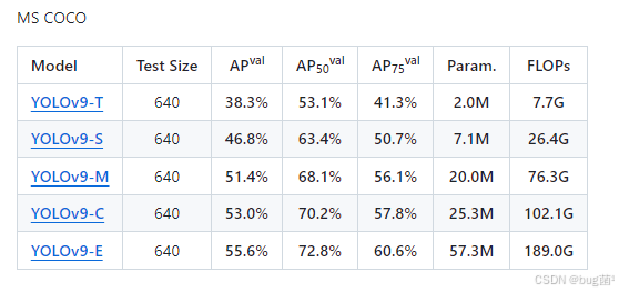
希望本文围绕 YOLOv9 的实战讲解,能够在以下几个维度上切实帮助到你:
- 🎯 模型精度提升:结合 YOLOv9 的 PGI、GELAN 等核心机制,从网络结构、特征融合、检测头、损失函数和数据增强等方向展开优化,通过工程实验提升目标检测精度;
- 🚀 推理速度优化:结合模型轻量化、结构重参数化、剪枝、量化、知识蒸馏与部署加速策略,帮助模型在真实业务场景中运行得更快、更稳定;
- 🧩 工程落地实践:覆盖数据准备、环境配置、模型训练、效果评估、问题排查、模型导出与部署推理等完整链路,提供可直接复用或稍加修改即可迁移的工程级方案;
- 🧠 核心机制理解:深入分析 YOLOv9 中可编程梯度信息与高效层聚合网络的设计逻辑,帮助你理解模型性能提升背后的原因,而不是停留在简单调用层面;
- 🔬 改进方案验证:通过消融实验、指标对比与可视化分析,评估不同改进模块对 Precision、Recall、mAP、FPS、参数量和计算量的实际影响。
PS:如果你按照文中步骤对 YOLOv9 进行优化后仍然遇到问题,请不必焦虑或灰心。
YOLOv9 是一个涉及网络结构、梯度传递、特征融合、训练策略与部署环境的复杂目标检测框架,最终表现会受到 硬件环境、数据集质量、任务定义、类别分布、训练配置、代码版本与部署平台 等多重因素的共同影响。
这是目标检测项目中十分常见的客观现象,并不代表你的操作存在问题,更不意味着某个改进模块一定无效。
如果你在实践过程中遇到以下问题:
- 🐛 模块替换后出现新的报错或 Bug;
- 📉 Precision、Recall 或 mAP 难以继续提升;
- 📈 训练损失异常、梯度不稳定或模型难以收敛;
- ⏱️ 推理速度、显存占用或部署性能不达预期;
- 🔄 修改网络结构后出现维度、通道数或特征层不匹配;
- 📦 模型导出 ONNX、TensorRT、OpenVINO 等格式时失败;
欢迎将 完整报错信息 + 环境版本 + 关键配置截图 + 网络配置文件 + 核心代码片段 粘贴至评论区,我们可以一起分析问题根因,并探讨更加可行的解决方案。
如果你已经摸索出更优的训练参数、网络结构、模块组合或部署优化思路,也非常欢迎在评论区分享。
你的每一条实战经验,都可能成为其他开发者解决问题、减少试错成本的关键线索。
部分章节还会结合国内外前沿论文与 AIGC 大模型技术,对 YOLOv9 的主流改进方案进行重构与再设计,使内容更加贴近工业检测、智慧交通、游戏分析、行为识别、遥感影像与边缘设备部署等真实应用场景。
🧧🧧 文末福利,等你来拿!🧧🧧
📌 文中所涉及的技术内容,大多来源于本人在 YOLOv9 项目中的一线实践积累,部分案例参考了开源项目、公开论文、技术社区资料与读者反馈。
如有版权相关问题,欢迎第一时间联系,我将尽快核实并进行修改或下线处理。
部分问题分析思路与排查路径参考了技术社区及 AI 问答平台,在此一并致谢 🙏
最后想说的是:
YOLOv9 的优化本质上是一个高度依赖任务、数据和部署环境的系统工程问题,不存在“一招通杀”的银弹方案。
PGI、GELAN、注意力机制、轻量化卷积、改进检测头、IoU 损失函数、特征融合模块和数据增强策略,都有其适用条件。
某个模块在公开数据集上取得提升,并不意味着它能够在所有自定义数据集、硬件平台和业务场景中获得同样收益。
真正有效的优化路径,永远源于:
- 对业务目标与评价指标的准确理解;
- 对数据质量和类别分布的持续分析;
- 对模型瓶颈的定位与针对性改进;
- 对实验变量的严格控制;
- 对精度、速度、参数量和部署成本的综合权衡;
- 以及一轮又一轮可复现的对比实验。
如果你已经在自己的项目中探索出了更加高效、稳定的 YOLOv9 优化路径,非常鼓励你:
- 💬 在评论区简要分享核心思路与实验结论;
- 📊 分享不同模块的消融实验结果;
- 📝 将完整过程整理成教程、博客或系列文章;
- 🔧 提交可复现的配置文件、代码或工程实践经验。
你的经验,或许正是别人卡关已久所缺少的最后一块拼图。
✅ 本期关于 YOLOv9 优化与实战应用 的内容就先聊到这里。
如果你想进一步深入:
- 🔍 系统理解 PGI、GELAN 与 YOLOv9 的整体网络结构;
- 🧱 学习主干网络、颈部网络、检测头与特征融合模块的改进方法;
- 📉 掌握损失函数、样本分配与训练策略的优化技巧;
- ⚡ 对比不同场景下的模型轻量化与部署加速方案;
- 🧪 建立规范的消融实验、指标对比与模型评估流程;
- 🧠 系统构建一套属于自己的 YOLOv9 调优方法论;
欢迎继续关注专栏:《YOLOv9实战:从入门到深度优化》
期待这些内容能够在你的项目中真正落地见效,帮助你 少踩坑、多提效、快验证、稳部署,我们下期见。
✨ 当然,如果 YOLOv9 专栏已经无法满足你,也可以继续关注:
-
《YOLOv10实战:从入门到深度优化》
-
《YOLOv11实战:从入门到深度优化》
更多新版本、新模块与新论文的工程复现内容,也会持续更新。
✍️ 码字不易,如果这篇文章对你有所启发或帮助,欢迎给我来个 一键三连:关注 + 点赞 + 收藏。
你的支持,是我持续输出高质量 YOLOv9 技术内容与工程实战案例最直接的动力来源。
同时诚挚推荐关注我的技术号: 「猿圈奇妙屋」
在这里,你可以:
- 📡 第一时间获取 YOLOv9、目标检测、多目标追踪与多任务学习等方向的进阶内容;
- 🛠️ 获取视觉算法、深度学习与模型部署的最新优化方案和工程实战经验;
- 📚 学习 PyTorch、OpenCV、ONNX、TensorRT 等相关技术;
- 🎁 获取 BAT 大厂面经、技术书籍 PDF、工程模板与常用工具清单等实用资源。
期待在更多维度上与你一起进步、共同成长。
🫵 Who am I?
我是专注于 计算机视觉、图像识别、目标检测与深度学习工程落地 的讲师和技术博主,笔名 bug菌:
- 活跃于 CSDN|稀土掘金|InfoQ|51CTO|华为云开发者社区|阿里云开发者社区|腾讯云开发者社区|开源中国|博客园|墨天轮 等技术社区;
- CSDN 博客之星 Top 30、华为云多年度十佳博主及卓越贡献奖获得者、掘金多年度人气作者 Top 40;
- CSDN、掘金、InfoQ、51CTO 等平台签约作者及优质创作者;
- 全网粉丝累计 30w+。
更多高质量技术内容与成长资料,可查看合集入口:
👉 点击查看 👈️
硬核技术号 「猿圈奇妙屋」 期待你的加入,一起进阶、一起打怪升级。

– End –