上一节
AI初学者指南 2
分类方法
Classify 使用的分类方法通常是自动选择的,但也可以进行修改。
将一些 2 D 坐标分类为颜色:

In[]:= Classify[colouredPoints, Method -> Automatic]
 添加时间目标选项:
In[]:= Classify[colouredPoints, Method -> Automatic, TimeGoal -> 30]

选择正确的方法
方法
一种常见的机器学习思维模式是不去问 “如何?” 或 “为什么?”,而是问 “它有效吗?”。
选择好方法的基本方法如下:
在数据的一个子集上测试每种方法。
选择给出最佳预测结果的方法。
将该方法应用于整个数据集。
1. 测试
In[]:= trainingData = ExampleData[{"MachineLearning", "FisherIris"}, "TrainingData"];
In[]:= testingData = ExampleData[{"MachineLearning", "FisherIris"}, "TestData"];
In[]:= SeedRandom[1];
In[]:= trainingSample = RandomSample[trainingData, 30]
Out[]= {{5.9, 3., 5.1, 1.8} -> "virginica", {5.8, 2.8, 5.1, 2.4} -> "virginica", {5.1, 3.3, 1.7, 0.5} -> "setosa", {4.7, 3.2, 1.3, 0.2} -> "setosa", {5.7, 2.9, 4.2, 1.3} -> "versicolor", {5.4, 3.9, 1.7, 0.4} -> "setosa", {5.8, 2.6, 4., 1.2} -> "versicolor", {4.9, 3.1, 1.5, 0.2} -> "setosa", {5.1, 2.5, 3., 1.1} -> "versicolor", {6.7, 2.5, 5.8, 1.8} -> "virginica", {4.8, 3.4, 1.9, 0.2} -> "setosa", {5., 3.2, 1.2, 0.2} -> "setosa", {5., 3.4, 1.5, 0.2} -> "setosa", {6.3, 2.8, 5.1, 1.5} -> "virginica", {6., 2.2, 5., 1.5} -> "virginica", {5.8, 2.7, 5.1, 1.9} -> "virginica", {4.6, 3.1, 1.5, 0.2} -> "setosa", {5., 3.5, 1.6, 0.6} -> "setosa", {5.6, 2.5, 3.9, 1.1} -> "versicolor", {5.5, 3.5, 1.3, 0.2} -> "setosa", {5.9, 3., 4.2, 1.5} -> "versicolor", {7.3, 2.9, 6.3, 1.8} -> "virginica", {5.7, 2.8, 4.1, 1.3} -> "versicolor", {5.5, 2.4, 3.7, 1.} -> "versicolor", {5.6, 3., 4.5, 1.5} -> "versicolor", {5., 3.5, 1.3, 0.3} -> "setosa", {6.7, 3.1, 5.6, 2.4} -> "virginica", {4.9, 3.6, 1.4, 0.1} -> "setosa", {6.8, 3., 5.5, 2.1} -> "virginica", {5.4, 3.9, 1.3, 0.4} -> "setosa"}
创建两个分类器,一个使用马尔可夫方法,另一个使用随机森林方法:
In[]:= irisClassifier1 = Classify[trainingSample, Method -> "Markov"];
In[]:= irisClassifier2 = Classify[trainingSample, Method -> "RandomForest"];
2. 选择
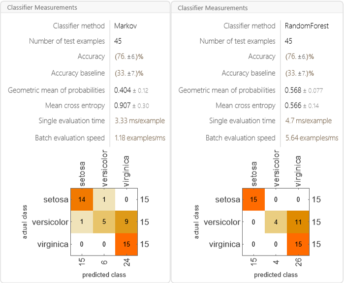
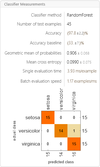
仅基于准确率来看,随机森林方法的表现往往更好:
In[]:= Row[{ClassifierMeasurements[irisClassifier1, testingData], ClassifierMeasurements[irisClassifier2, testingData]}]
3. 应用
将随机森林方法应用于整个训练数据集:
In[]:= irisClassifier3 = Classify[trainingData, Method -> "RandomForest"]

检查准确率:
In[]:= ClassifierMeasurements[irisClassifier3, testingData]
预测
一旦模型在某些数据上经过训练,它就可以用来预测新的数据值。
这在填补缺失数据点 (这一过程称为插补) 时特别有用。
预测
获取马萨诸塞州波士顿的房屋数据:
In[]:= homeData = ResourceData["Sample Data: Boston Homes"];
查看列标题及其描述:
In[]:= Thread[Values[ResourceData["Sample Data: Boston Homes", {"ColumnHeadings", "ColumnDescriptions"}]]] // Dataset
| CRIM | Per capita crime rate by town |
| ZN | Proportion of residential land zoned for lots over 25000 square feet |
| INDUS | Proportion of non-retail business acres per town |
| CHAS | Charles River dummy variable (1 if tract bounds river, 0 otherwise) |
| NOX | Nitrogen oxide concentration (parts per 10 million) |
| RM | Average number of rooms per dwelling |
| AGE | Proportion of owner-occupied units built prior to 1940 |
| DIS | Weighted mean of distances to five Boston employment centers |
| RAD | Index of accessibility to radial highways |
| TAX | Full-value property-tax rater per $10000 |
| PTRATIO | Pupil-teacher ratio by town |
| BLACK | 1000(Bk-0.63)^2 where Bk is the proportion of Black or African-American residents by town |
| LSTAT | Lower status of the population (percent) |
| MEDV | Median value of owner-occupied homes in $1000s |
假设你想根据房屋的其他特征来预测其价值 (即 MEDV 列)。
将数据拆分为训练集和测试集,然后创建一个预测器:
In[]:= trainingData = RandomSample[homeData][[;; 400]];
testingData = RandomSample[homeData][[401 ;;]];
In[]:= predictor = Predict[trainingData -> "MEDV", PerformanceGoal -> "Quality"]
In[]:= predictor = Predict[trainingData -> "MEDV", PerformanceGoal -> "Quality"]

使用预测器来估算缺失的房屋价格 (单位:千美元):

Out[]= 10.4
从预测器获取测量结果:
In[]:= predictorMeasurements = PredictorMeasurements[predictor, testingData -> "MEDV"]
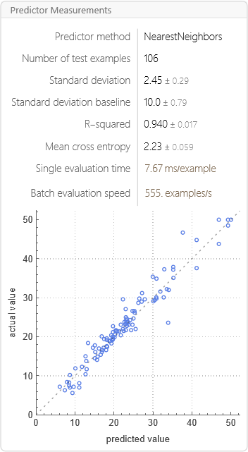 从上图可以看到预测自动选择了KNN最近邻方法。