第七十九篇:电磁场不确定性量化与可靠性分析
摘要
电磁场不确定性量化与可靠性分析是评估电磁器件在不确定因素影响下性能波动和失效风险的重要方法。本主题系统介绍不确定性量化的基本理论、概率统计方法、不确定性传播技术以及可靠性评估方法。重点阐述蒙特卡洛模拟、多项式混沌展开、随机配点法等不确定性传播方法,探讨电磁场仿真中材料参数、几何尺寸、边界条件等不确定性来源的建模方法。通过Python实现微波器件、天线系统、电磁兼容等典型应用的不确定性量化和可靠性分析,展示从输入不确定性到输出响应统计特性的完整传播过程,为电磁器件的稳健设计和风险评估提供理论指导和工程实践方法。
关键词
不确定性量化,可靠性分析,蒙特卡洛模拟,多项式混沌展开,随机配点法,敏感性分析,失效概率,稳健设计
1. 不确定性量化基础理论
1.1 不确定性来源与分类
电磁场仿真中的不确定性来源:
材料参数不确定性:
- 介电常数 ε\\varepsilonε 的制造公差
- 磁导率 μ\\muμ 的频率依赖性
- 电导率 σ\\sigmaσ 的温度敏感性
几何尺寸不确定性:
- 加工精度限制导致的尺寸偏差
- 装配误差引起的间隙变化
- 热膨胀导致的形变
边界条件不确定性:
- 端口阻抗的容差
- 激励源的幅度和相位波动
- 环境电磁干扰
模型不确定性:
- 数值模型的近似误差
- 物理模型的简化假设
- 网格离散化误差
不确定性分类:
不确定性={偶然不确定性(Aleatory)固有的随机性认知不确定性(Epistemic)知识缺乏导致的\\text{不确定性} = \\begin{cases}
\\text{偶然不确定性(Aleatory)} & \\text{固有的随机性} \\\\
\\text{认知不确定性(Epistemic)} & \\text{知识缺乏导致的}
\\end{cases}不确定性={偶然不确定性(Aleatory)认知不确定性(Epistemic)固有的随机性知识缺乏导致的
1.2 概率建模基础
随机变量表示:
电磁参数表示为随机变量:
ε(ξ)=εˉ+σεξ\\varepsilon(\\xi) = \\bar{\\varepsilon} + \\sigma_\\varepsilon \\xiε(ξ)=εˉ+σεξ
其中 ξ\\xiξ 为标准随机变量,εˉ\\bar{\\varepsilon}εˉ 为均值,σε\\sigma_\\varepsilonσε 为标准差。
常用概率分布:
正态分布:
f(x)=12πσexp(−(x−μ)22σ2)f(x) = \\frac{1}{\\sqrt{2\\pi}\\sigma} \\exp\\left(-\\frac{(x-\\mu)^2}{2\\sigma^2}\\right)f(x)=2πσ1exp(−2σ2(x−μ)2)
均匀分布:
f(x)={1b−aa≤x≤b0otherwisef(x) = \\begin{cases} \\frac{1}{b-a} & a \\leq x \\leq b \\\\ 0 & \\text{otherwise} \\end{cases}f(x)={b−a10a≤x≤botherwise
对数正态分布:
f(x)=1xσ2πexp(−(lnx−μ)22σ2)f(x) = \\frac{1}{x\\sigma\\sqrt{2\\pi}} \\exp\\left(-\\frac{(\\ln x – \\mu)^2}{2\\sigma^2}\\right)f(x)=xσ2π1exp(−2σ2(lnx−μ)2)
威布尔分布:
f(x)=kλ(xλ)k−1exp(−(xλ)k)f(x) = \\frac{k}{\\lambda}\\left(\\frac{x}{\\lambda}\\right)^{k-1} \\exp\\left(-\\left(\\frac{x}{\\lambda}\\right)^k\\right)f(x)=λk(λx)k−1exp(−(λx)k)
1.3 不确定性传播问题
数学描述:
给定输入随机向量 X=(X1,X2,…,Xn)\\mathbf{X} = (X_1, X_2, …, X_n)X=(X1,X2,…,Xn),输出响应:
Y=f(X)Y = f(\\mathbf{X})Y=f(X)
不确定性传播的目标是确定输出 YYY 的统计特性:
- 均值 μY=E[Y]\\mu_Y = E[Y]μY=E[Y]
- 方差 σY2=E[(Y−μY)2]\\sigma_Y^2 = E[(Y – \\mu_Y)^2]σY2=E[(Y−μY)2]
- 概率密度函数 fY(y)f_Y(y)fY(y)
- 累积分布函数 FY(y)F_Y(y)FY(y)
2. 蒙特卡洛模拟方法
2.1 基本蒙特卡洛方法
算法流程:
μ^Y=1N∑i=1NY(i)\\hat{\\mu}_Y = \\frac{1}{N} \\sum_{i=1}^{N} Y^{(i)}μ^Y=N1i=1∑NY(i)
σ^Y2=1N−1∑i=1N(Y(i)−μ^Y)2\\hat{\\sigma}_Y^2 = \\frac{1}{N-1} \\sum_{i=1}^{N} (Y^{(i)} – \\hat{\\mu}_Y)^2σ^Y2=N−11i=1∑N(Y(i)−μ^Y)2
收敛性分析:
蒙特卡洛估计的误差:
RMSE=σYN\\text{RMSE} = \\frac{\\sigma_Y}{\\sqrt{N}}RMSE=NσY
误差以 O(N−1/2)O(N^{-1/2})O(N−1/2) 的速度收敛,与维度无关。
2.2 方差缩减技术
重要性采样:
E[Y]=∫f(x)fX(x)g(x)g(x)dxE[Y] = \\int f(\\mathbf{x}) \\frac{f_\\mathbf{X}(\\mathbf{x})}{g(\\mathbf{x})} g(\\mathbf{x}) d\\mathbf{x}E[Y]=∫f(x)g(x)fX(x)g(x)dx
其中 g(x)g(\\mathbf{x})g(x) 为重要性密度函数。
拉丁超立方采样(LHS):
将每个维度分成 NNN 个等概率区间,在每个区间中随机采样一个点,保证样本的均匀分布。
拟蒙特卡洛方法:
使用低差异序列(如Sobol序列)代替伪随机数:
DN∗=O((logN)dN)D_N^* = O\\left(\\frac{(\\log N)^d}{N}\\right)DN∗=O(N(logN)d)
2.3 分层采样
分层蒙特卡洛:
将样本空间划分为 KKK 层,每层独立采样:
μ^Y=∑k=1Kwkμ^k\\hat{\\mu}_Y = \\sum_{k=1}^{K} w_k \\hat{\\mu}_kμ^Y=k=1∑Kwkμ^k
其中 wkw_kwk 为第 kkk 层的权重。
3. 谱不确定性量化方法
3.1 多项式混沌展开(PCE)
基本理论:
将随机输出展开为随机变量的多项式级数:
Y(ξ)=∑α∈AyαΨα(ξ)Y(\\xi) = \\sum_{\\alpha \\in \\mathcal{A}} y_\\alpha \\Psi_\\alpha(\\xi)Y(ξ)=α∈A∑yαΨα(ξ)
其中 Ψα(ξ)\\Psi_\\alpha(\\xi)Ψα(ξ) 为正交多项式,α\\alphaα 为多指标。
正交多项式选择:
| 正态分布 | Hermite | e−ξ2/2e^{-\\xi^2/2}e−ξ2/2 |
| 均匀分布 | Legendre | 1 |
| Gamma分布 | Laguerre | e−ξe^{-\\xi}e−ξ |
| Beta分布 | Jacobi | (1−ξ)α(1+ξ)β(1-\\xi)^\\alpha(1+\\xi)^\\beta(1−ξ)α(1+ξ)β |
统计矩计算:
均值:μY=y0\\mu_Y = y_0μY=y0
方差:σY2=∑α≠0yα2⟨Ψα2⟩\\sigma_Y^2 = \\sum_{\\alpha \\neq 0} y_\\alpha^2 \\langle \\Psi_\\alpha^2 \\rangleσY2=∑α=0yα2⟨Ψα2⟩
3.2 随机配点法
基本思想:
在精心选择的配点上求解确定性问题,通过插值获得统计特性。
配点选择:
- 张量积配点:ξi⊗ξj\\xi_i \\otimes \\xi_jξi⊗ξj
- 稀疏网格配点:Smolyak算法
- 高斯积分点:与正交多项式对应
插值方法:
Y(ξ)≈∑i=1NY(ξ(i))Li(ξ)Y(\\xi) \\approx \\sum_{i=1}^{N} Y(\\xi^{(i)}) L_i(\\xi)Y(ξ)≈i=1∑NY(ξ(i))Li(ξ)
其中 Li(ξ)L_i(\\xi)Li(ξ) 为Lagrange插值基函数。
3.3 降维技术
主成分分析(PCA):
X=μ+Wξ\\mathbf{X} = \\boldsymbol{\\mu} + \\mathbf{W} \\boldsymbol{\\xi}X=μ+Wξ
其中 W\\mathbf{W}W 为特征向量矩阵,ξ\\boldsymbol{\\xi}ξ 为降维后的随机变量。
Karhunen-Loève展开:
对于随机场:
X(r,ω)=Xˉ(r)+∑i=1∞λiϕi(r)ξi(ω)X(\\mathbf{r}, \\omega) = \\bar{X}(\\mathbf{r}) + \\sum_{i=1}^{\\infty} \\sqrt{\\lambda_i} \\phi_i(\\mathbf{r}) \\xi_i(\\omega)X(r,ω)=Xˉ(r)+i=1∑∞λiϕi(r)ξi(ω)
4. 敏感性分析方法
4.1 局部敏感性分析
偏导数法:
Si=∂Y∂Xi∣X=μS_i = \\frac{\\partial Y}{\\partial X_i}\\bigg|_{\\mathbf{X}=\\boldsymbol{\\mu}}Si=∂Xi∂YX=μ
标准化敏感性:
Sinorm=σXiσY∂Y∂XiS_i^{\\text{norm}} = \\frac{\\sigma_{X_i}}{\\sigma_Y} \\frac{\\partial Y}{\\partial X_i}Sinorm=σYσXi∂Xi∂Y
4.2 全局敏感性分析
Sobol指数:
一阶Sobol指数:
Si=VXi(EX∼i[Y∣Xi])V(Y)S_i = \\frac{V_{X_i}(E_{\\mathbf{X}_{\\sim i}}[Y|X_i])}{V(Y)}Si=V(Y)VXi(EX∼i[Y∣Xi])
总效应指数:
SiT=EX∼i[VXi(Y∣X∼i)]V(Y)S_i^T = \\frac{E_{\\mathbf{X}_{\\sim i}}[V_{X_i}(Y|\\mathbf{X}_{\\sim i})]}{V(Y)}SiT=V(Y)EX∼i[VXi(Y∣X∼i)]
Morris筛选法:
通过计算基本效应的统计量识别重要参数:
EEi=Y(x1,…,xi+Δ,…,xn)−Y(x)ΔEE_i = \\frac{Y(x_1, …, x_i + \\Delta, …, x_n) – Y(\\mathbf{x})}{\\Delta}EEi=ΔY(x1,…,xi+Δ,…,xn)−Y(x)
4.3 基于PCE的敏感性分析
主敏感性指数:
Si=∑α∈Aiyα2⟨Ψα2⟩σY2S_i = \\frac{\\sum_{\\alpha \\in \\mathcal{A}_i} y_\\alpha^2 \\langle \\Psi_\\alpha^2 \\rangle}{\\sigma_Y^2}Si=σY2∑α∈Aiyα2⟨Ψα2⟩
其中 Ai\\mathcal{A}_iAi 为仅依赖于 XiX_iXi 的多指标集合。
5. 可靠性分析方法
5.1 失效概率计算
定义:
失效概率:
Pf=P(g(X)≤0)=∫g(x)≤0fX(x)dxP_f = P(g(\\mathbf{X}) \\leq 0) = \\int_{g(\\mathbf{x}) \\leq 0} f_\\mathbf{X}(\\mathbf{x}) d\\mathbf{x}Pf=P(g(X)≤0)=∫g(x)≤0fX(x)dx
其中 g(X)g(\\mathbf{X})g(X) 为极限状态函数。
蒙特卡洛估计:
P^f=1N∑i=1NI(g(X(i))≤0)\\hat{P}_f = \\frac{1}{N} \\sum_{i=1}^{N} I(g(\\mathbf{X}^{(i)}) \\leq 0)P^f=N1i=1∑NI(g(X(i))≤0)
其中 I(⋅)I(\\cdot)I(⋅) 为指示函数。
5.2 一阶可靠性方法(FORM)
基本思想:
将随机变量变换到标准正态空间,寻找设计点(最可能失效点)。
Hasofer-Lind可靠性指标:
β=ming(u)=0∥u∥\\beta = \\min_{g(\\mathbf{u})=0} \\|\\mathbf{u}\\|β=g(u)=0min∥u∥
失效概率近似:
Pf≈Φ(−β)P_f \\approx \\Phi(-\\beta)Pf≈Φ(−β)
迭代算法:
5.3 二阶可靠性方法(SORM)
曲率修正:
Pf≈Φ(−β)∏i=1n−1(1+βκi)−1/2P_f \\approx \\Phi(-\\beta) \\prod_{i=1}^{n-1} (1 + \\beta \\kappa_i)^{-1/2}Pf≈Φ(−β)i=1∏n−1(1+βκi)−1/2
其中 κi\\kappa_iκi 为极限状态函数在设计点处的主曲率。
5.4 重要性抽样可靠性分析
最优重要性密度:
g∗(x)=I(g(x)≤0)fX(x)Pfg^*(\\mathbf{x}) = \\frac{I(g(\\mathbf{x}) \\leq 0) f_\\mathbf{X}(\\mathbf{x})}{P_f}g∗(x)=PfI(g(x)≤0)fX(x)
设计点中心法:
以FORM找到的设计点为中心构建重要性密度。
6. 稳健设计优化
6.1 稳健性指标
信噪比:
SN=10log10(μY2σY2)SN = 10 \\log_{10}\\left(\\frac{\\mu_Y^2}{\\sigma_Y^2}\\right)SN=10log10(σY2μY2)
性能指数:
PI=μY−TσYPI = \\frac{\\mu_Y – T}{\\sigma_Y}PI=σYμY−T
其中 TTT 为目标值。
6.2 双响应面法
均值和方差模型:
μ^Y=fμ(x)\\hat{\\mu}_Y = f_\\mu(\\mathbf{x})μ^Y=fμ(x)
σ^Y=fσ(x)\\hat{\\sigma}_Y = f_\\sigma(\\mathbf{x})σ^Y=fσ(x)
优化问题:
minxσ^Ys.t.μ^Y=T\\min_{\\mathbf{x}} \\hat{\\sigma}_Y \\quad \\text{s.t.} \\quad \\hat{\\mu}_Y = Txminσ^Ys.t.μ^Y=T
6.3 基于可靠性的设计优化(RBDO)
数学模型:
mindC(d)\\min_{\\mathbf{d}} C(\\mathbf{d})dminC(d)
s.t.P(gi(X)≤0)≤Pf,itarget,i=1,…,m\\text{s.t.} \\quad P(g_i(\\mathbf{X}) \\leq 0) \\leq P_{f,i}^{target}, \\quad i = 1, …, ms.t.P(gi(X)≤0)≤Pf,itarget,i=1,…,m
可靠性约束处理:
- 性能度量法(PMA)
- 可靠性指标法(RIA)
- 顺序优化与可靠性评估(SORA)
7. 工程应用
7.1 微波器件容差分析
应用场景:
- 滤波器频率响应的容差分析
- 功分器功率分配的波动评估
- 耦合器隔离度的可靠性验证
7.2 天线性能稳健性
应用场景:
- 天线增益的制造敏感性
- 辐射方向图的稳定性
- 阻抗带宽的可靠性
7.3 电磁兼容可靠性
应用场景:
- 屏蔽效能的置信区间
- 辐射发射的合规概率
- 敏感度阈值的不确定性
8. 案例研究
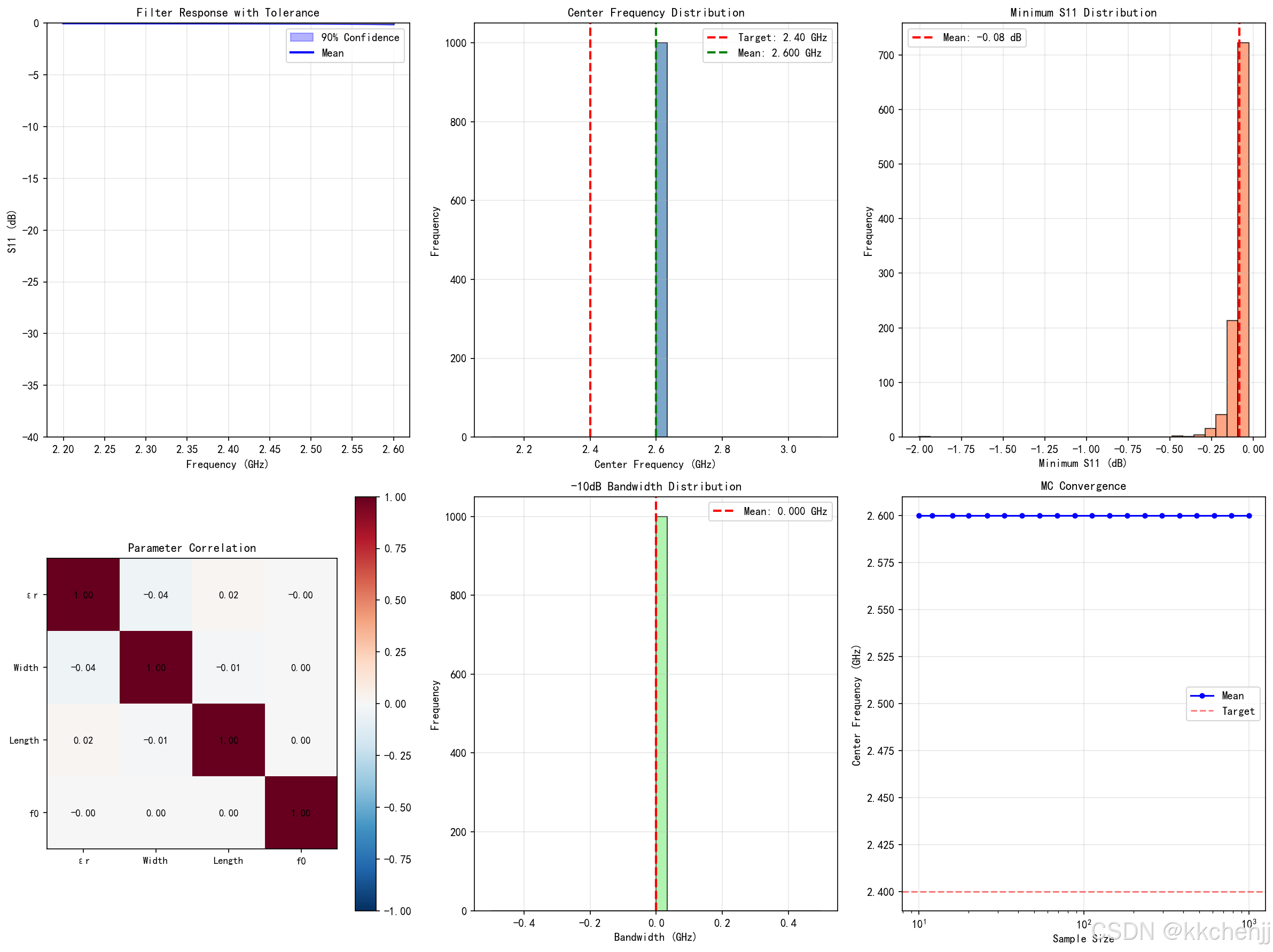
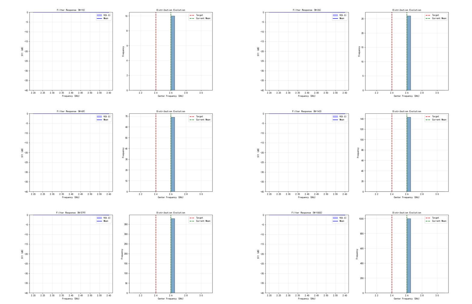
8.1 案例1:微带滤波器容差分析(含GIF动画)
分析基板介电常数和线宽公差对滤波器S参数的影响。
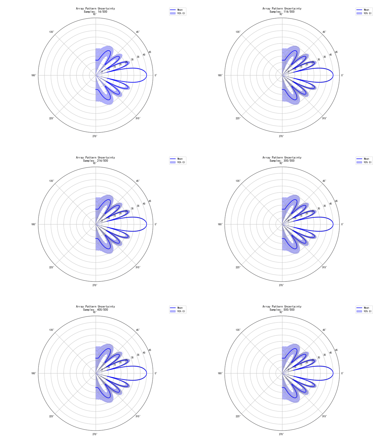
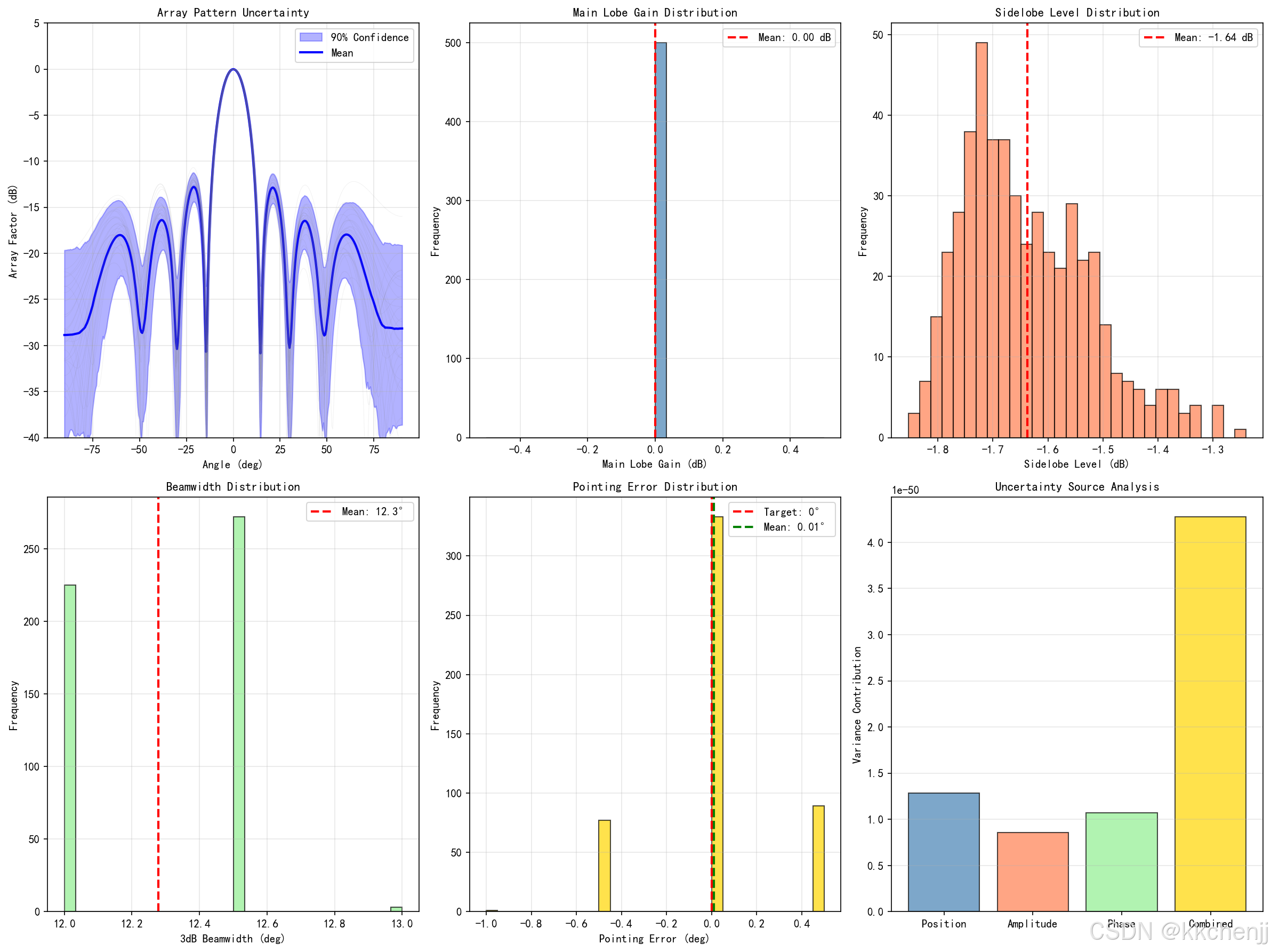
8.2 案例2:天线阵列方向图不确定性(含GIF动画)
评估阵元位置误差和激励相位误差对方向图的影响。
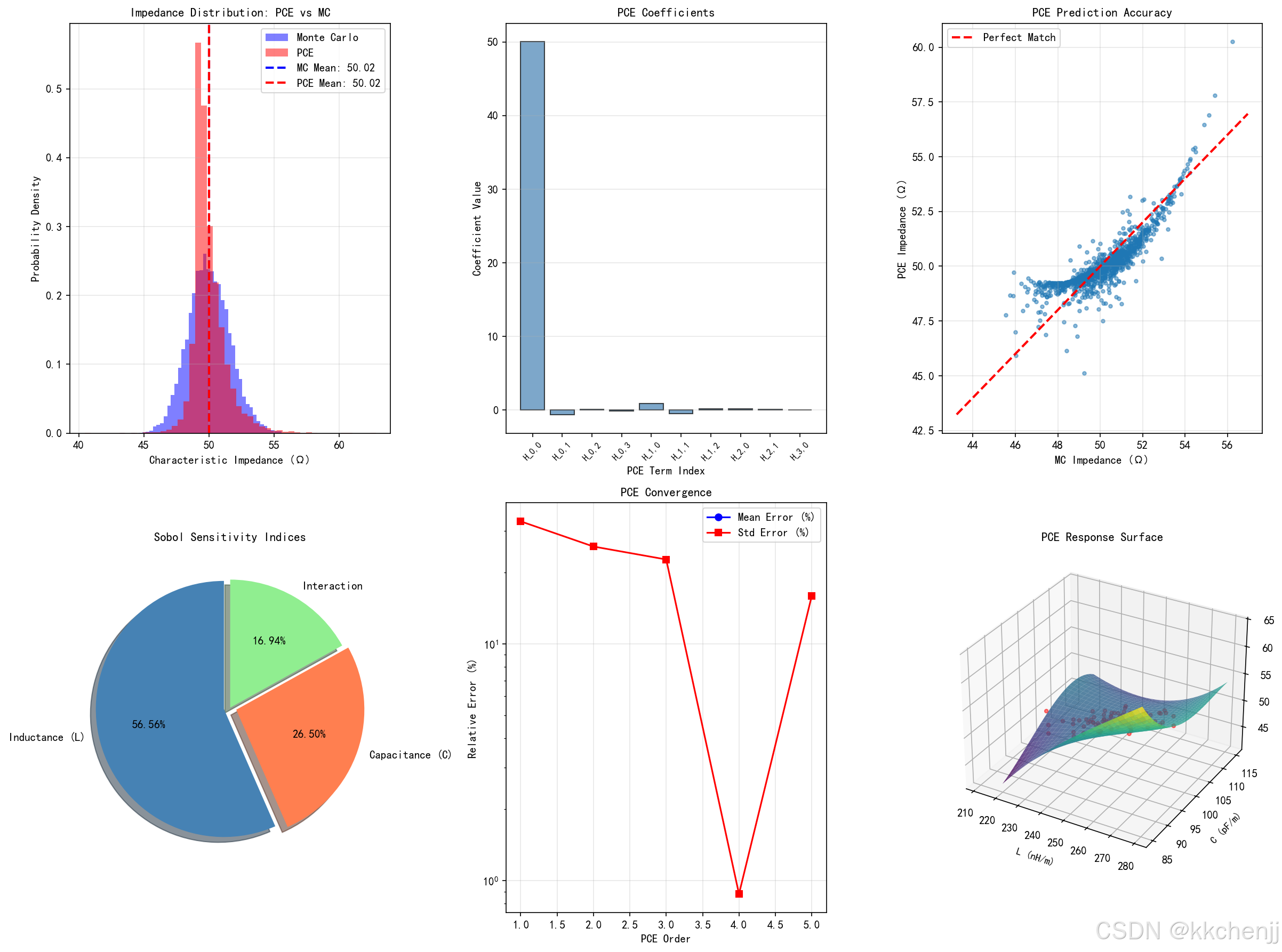
8.3 案例3:多项式混沌展开应用
使用PCE方法高效计算微波器件的统计特性。
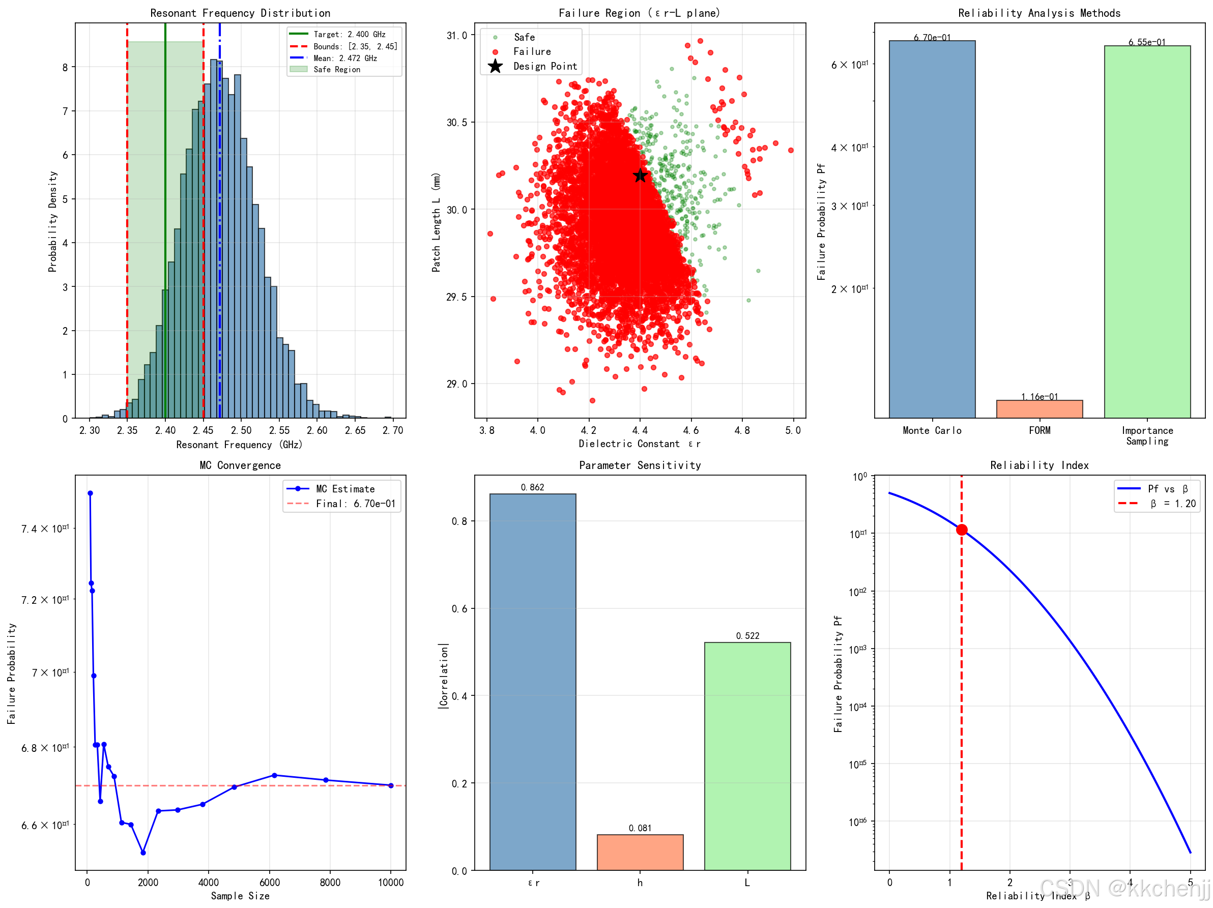
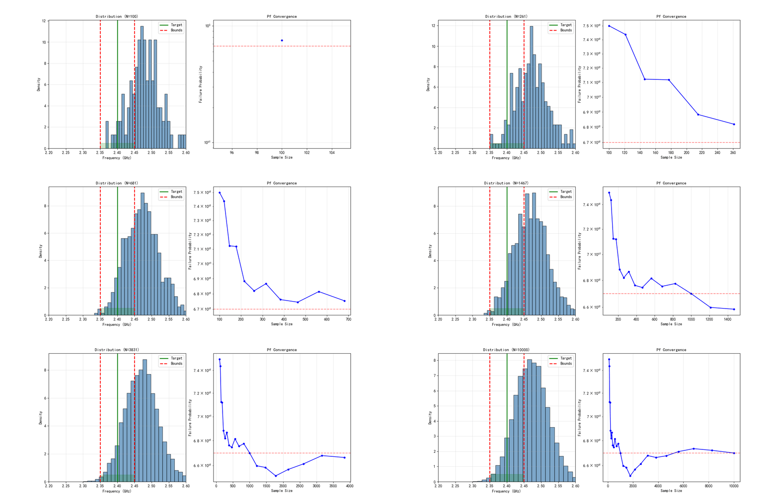
8.4 案例4:可靠性分析与失效概率计算(含GIF动画)
计算电磁器件的失效概率和可靠性指标。
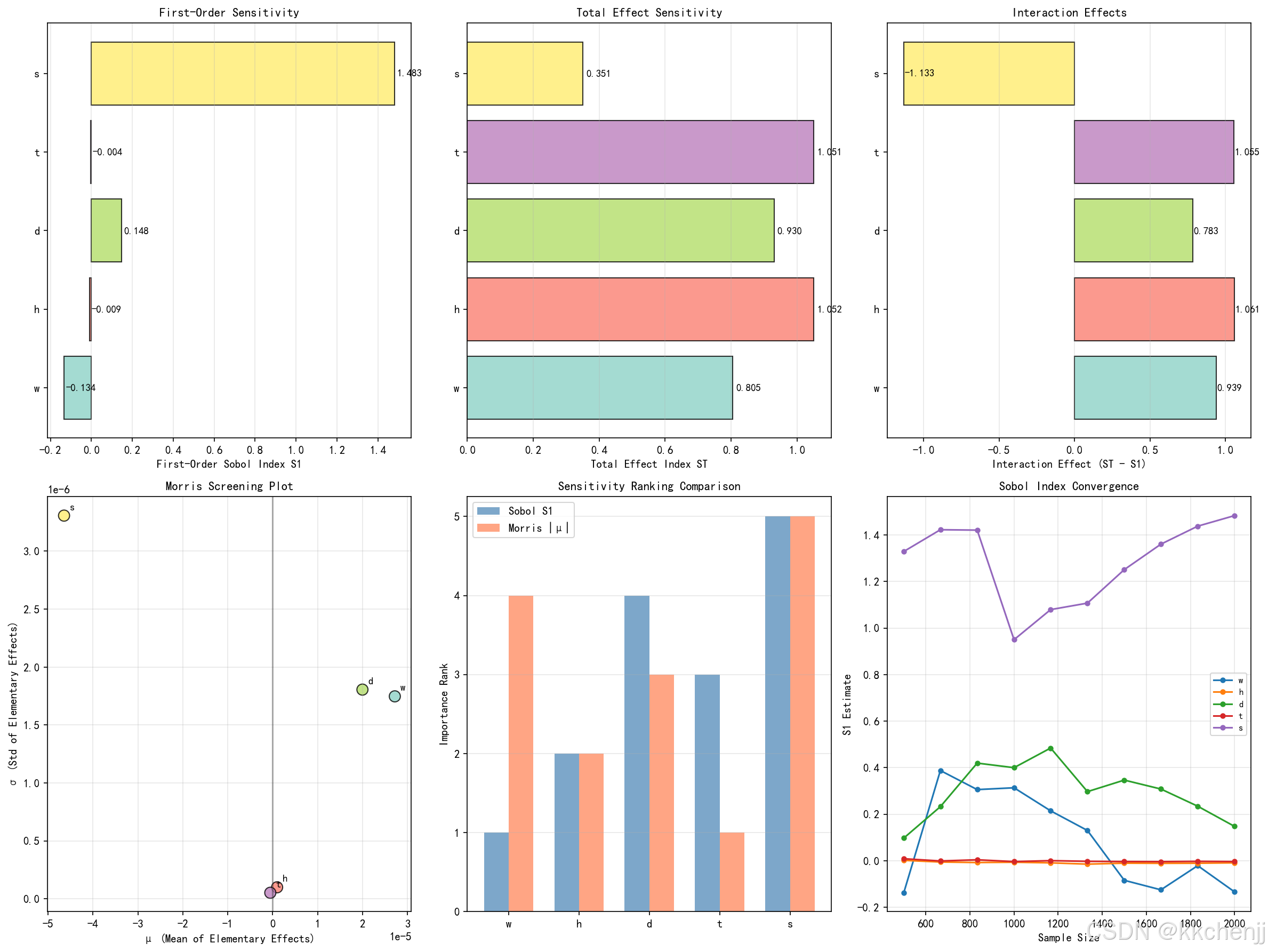
8.5 案例5:全局敏感性分析
使用Sobol指数识别影响电磁性能的关键参数。
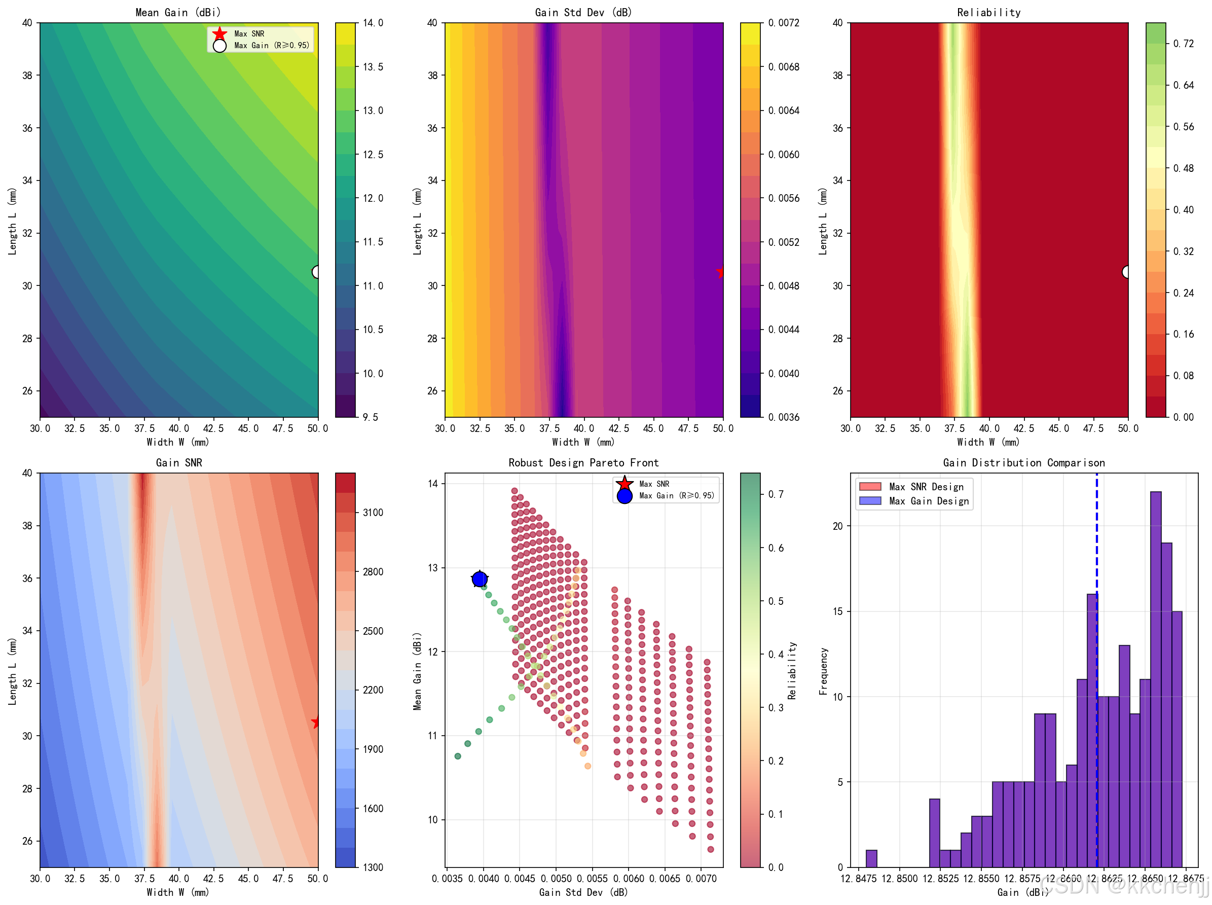
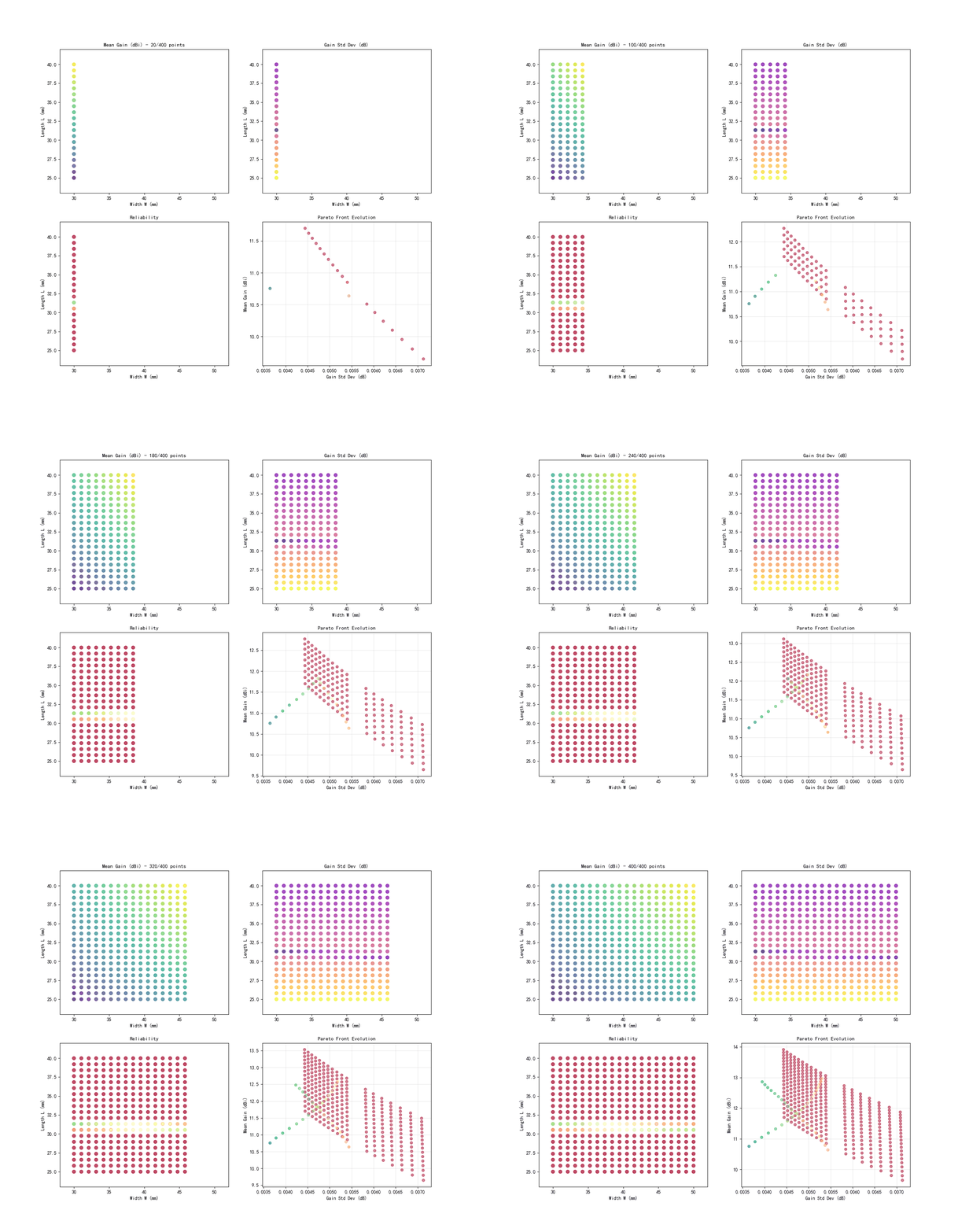
8.6 案例6:稳健设计优化(含GIF动画)
优化设计参数以最小化性能波动。
9. 结果分析与讨论
9.1 方法对比
- 蒙特卡洛 vs PCE vs 随机配点法
- 计算效率与精度的权衡
- 不同维度问题的适用性
9.2 参数影响分析
- 样本数量对收敛性的影响
- 多项式阶数对PCE精度的影响
- 稀疏网格水平对计算成本的影响
9.3 工程实践建议
- 不确定性建模的最佳实践
- 计算资源与精度要求的平衡
- 验证与确认方法
10. 扩展应用
10.1 多物理场不确定性量化
考虑电磁-热-结构耦合的不确定性传播。
10.2 时域不确定性分析
瞬态电磁场问题的随机分析。
10.3 深度学习辅助UQ
使用神经网络替代传统仿真加速不确定性量化。
11. 总结与展望
本主题系统介绍了电磁场不确定性量化与可靠性分析的理论基础和方法体系:
核心理论:
- 不确定性来源识别与概率建模
- 蒙特卡洛模拟及其方差缩减技术
- 谱方法(PCE、随机配点法)
- 敏感性分析方法
可靠性方法:
- FORM/SORM方法
- 重要性抽样技术
- 基于可靠性的设计优化
工程应用:
- 微波器件、天线、电磁兼容
- 容差分析、稳健设计、风险评估
未来发展方向:
不确定性量化与可靠性分析为电磁器件的稳健设计和风险评估提供了科学方法,能够有效降低设计风险,提高产品可靠性。
参考文献
R. G. Ghanem, P. D. Spanos. Stochastic Finite Elements: A Spectral Approach. Dover, 2003.
D. Xiu. Numerical Methods for Stochastic Computations: A Spectral Method Approach. Princeton University Press, 2010.
T. J. Sullivan. Introduction to Uncertainty Quantification. Springer, 2015.
A. Der Kiureghian. First- and second-order reliability methods. Engineering Safety, 2000.
I. M. Sobol. Global sensitivity indices for nonlinear mathematical models. Mathematical Modeling and Computational Experiment, 1993.
B. Sudret. Global sensitivity analysis using polynomial chaos expansions. Reliability Engineering & System Safety, 2008.
S. K. Au, J. L. Beck. Estimation of small failure probabilities in high dimensions by subset simulation. Probabilistic Engineering Mechanics, 2001.
康顺, 等. 不确定性量化方法及其应用. 科学出版社, 2018.
附录:Python代码清单
# -*- coding: utf-8 -*-
"""
主题079:电磁场不确定性量化与可靠性分析仿真
包含6个案例:
1. 微带滤波器容差分析(含GIF动画)
2. 天线阵列方向图不确定性(含GIF动画)
3. 多项式混沌展开应用
4. 可靠性分析与失效概率计算(含GIF动画)
5. 全局敏感性分析
6. 稳健设计优化(含GIF动画)
"""
import matplotlib
matplotlib.use('Agg')
import numpy as np
import matplotlib.pyplot as plt
from matplotlib.animation import FuncAnimation, PillowWriter
from matplotlib.patches import Rectangle, Circle, FancyBboxPatch
from scipy import stats, optimize
from scipy.special import erf, erfc
import warnings
warnings.filterwarnings('ignore')
import os
# 创建输出目录
output_dir = r'd:\\文档\\500仿真领域\\工程仿真\\电磁场耦合仿真\\主题079_电磁场不确定性量化与可靠性分析'
os.makedirs(output_dir, exist_ok=True)
# 设置中文字体
plt.rcParams['font.sans-serif'] = ['SimHei', 'DejaVu Sans']
plt.rcParams['axes.unicode_minus'] = False
print("=" * 70)
print("主题079:电磁场不确定性量化与可靠性分析仿真")
print("=" * 70)
print("\\n开始运行不确定性量化与可靠性分析仿真案例…")
print("=" * 70)
# =============================================================================
# 案例1:微带滤波器容差分析(含GIF动画)
# =============================================================================
def case1_filter_tolerance():
"""案例1:微带滤波器容差分析"""
print("\\n案例1:微带滤波器容差分析")
print("-" * 60)
# 滤波器参数
f0 = 2.4e9 # 中心频率2.4GHz
BW = 0.1 # 相对带宽10%
# 不确定性参数
# 基板介电常数:标称值4.4,标准差0.1
eps_mean = 4.4
eps_std = 0.1
# 线宽:标称值1.0mm,标准差0.05mm
w_mean = 1.0
w_std = 0.05
# 线长:标称值30mm,标准差0.5mm
l_mean = 30.0
l_std = 0.5
# 蒙特卡洛采样
n_samples = 1000
np.random.seed(42)
eps_samples = np.random.normal(eps_mean, eps_std, n_samples)
w_samples = np.random.normal(w_mean, w_std, n_samples)
l_samples = np.random.normal(l_mean, l_std, n_samples)
print(f" 执行蒙特卡洛模拟 (N={n_samples})…")
# 计算S11参数(简化模型)
# S11与频率、介电常数、线宽、线长相关
freq = np.linspace(2.2e9, 2.6e9, 100)
S11_samples = np.zeros((n_samples, len(freq)))
for i in range(n_samples):
# 简化的滤波器响应模型
# 有效介电常数
eps_eff = (eps_samples[i] + 1) / 2 + (eps_samples[i] – 1) / (2 * np.sqrt(1 + 12 * w_samples[i]))
# 谐振频率偏移
f_res = f0 * np.sqrt(eps_mean / eps_eff) * (l_mean / l_samples[i])
# S11响应(简化模型)
Q = 50 # 品质因数
for j, f in enumerate(freq):
detuning = (f – f_res) / (f_res / (2 * Q))
S11_samples[i, j] = –20 * np.log10(np.sqrt(1 + 1/(detuning**2 + 1e-10)))
# 统计分析
S11_mean = np.mean(S11_samples, axis=0)
S11_std = np.std(S11_samples, axis=0)
S11_p5 = np.percentile(S11_samples, 5, axis=0)
S11_p95 = np.percentile(S11_samples, 95, axis=0)
# 创建可视化
fig = plt.figure(figsize=(16, 12))
# S11响应及置信区间
ax1 = fig.add_subplot(2, 3, 1)
ax1.fill_between(freq/1e9, S11_p5, S11_p95, alpha=0.3, color='blue', label='90% Confidence')
ax1.plot(freq/1e9, S11_mean, 'b-', linewidth=2, label='Mean')
for i in range(min(50, n_samples)):
ax1.plot(freq/1e9, S11_samples[i], 'gray', alpha=0.1, linewidth=0.5)
ax1.set_xlabel('Frequency (GHz)', fontsize=10)
ax1.set_ylabel('S11 (dB)', fontsize=10)
ax1.set_title('Filter Response with Tolerance', fontsize=11, fontweight='bold')
ax1.legend()
ax1.grid(True, alpha=0.3)
ax1.set_ylim(–40, 0)
# 中心频率分布
ax2 = fig.add_subplot(2, 3, 2)
f_center_samples = freq[np.argmin(S11_samples, axis=1)]
ax2.hist(f_center_samples/1e9, bins=30, color='steelblue', edgecolor='black', alpha=0.7)
ax2.axvline(f0/1e9, color='red', linestyle='–', linewidth=2, label=f'Target: {f0/1e9:.2f} GHz')
ax2.axvline(np.mean(f_center_samples)/1e9, color='green', linestyle='–', linewidth=2,
label=f'Mean: {np.mean(f_center_samples)/1e9:.3f} GHz')
ax2.set_xlabel('Center Frequency (GHz)', fontsize=10)
ax2.set_ylabel('Frequency', fontsize=10)
ax2.set_title('Center Frequency Distribution', fontsize=11, fontweight='bold')
ax2.legend()
ax2.grid(True, alpha=0.3)
# 最小S11分布
ax3 = fig.add_subplot(2, 3, 3)
S11_min_samples = np.min(S11_samples, axis=1)
ax3.hist(S11_min_samples, bins=30, color='coral', edgecolor='black', alpha=0.7)
ax3.axvline(np.mean(S11_min_samples), color='red', linestyle='–', linewidth=2,
label=f'Mean: {np.mean(S11_min_samples):.2f} dB')
ax3.set_xlabel('Minimum S11 (dB)', fontsize=10)
ax3.set_ylabel('Frequency', fontsize=10)
ax3.set_title('Minimum S11 Distribution', fontsize=11, fontweight='bold')
ax3.legend()
ax3.grid(True, alpha=0.3)
# 参数相关性分析
ax4 = fig.add_subplot(2, 3, 4)
correlation_matrix = np.corrcoef([eps_samples, w_samples, l_samples, f_center_samples/1e9])
im = ax4.imshow(correlation_matrix, cmap='RdBu_r', vmin=–1, vmax=1)
ax4.set_xticks(range(4))
ax4.set_yticks(range(4))
ax4.set_xticklabels(['εr', 'Width', 'Length', 'f0'], fontsize=9)
ax4.set_yticklabels(['εr', 'Width', 'Length', 'f0'], fontsize=9)
for i in range(4):
for j in range(4):
ax4.text(j, i, f'{correlation_matrix[i,j]:.2f}', ha='center', va='center', fontsize=9)
ax4.set_title('Parameter Correlation', fontsize=11, fontweight='bold')
plt.colorbar(im, ax=ax4)
# 带宽分布
ax5 = fig.add_subplot(2, 3, 5)
# 计算-10dB带宽
BW_samples = []
for i in range(n_samples):
idx = np.where(S11_samples[i] < –10)[0]
if len(idx) > 1:
BW_samples.append((freq[idx[–1]] – freq[idx[0]]) / 1e9)
else:
BW_samples.append(0)
BW_samples = np.array(BW_samples)
ax5.hist(BW_samples, bins=30, color='lightgreen', edgecolor='black', alpha=0.7)
ax5.axvline(np.mean(BW_samples), color='red', linestyle='–', linewidth=2,
label=f'Mean: {np.mean(BW_samples):.3f} GHz')
ax5.set_xlabel('Bandwidth (GHz)', fontsize=10)
ax5.set_ylabel('Frequency', fontsize=10)
ax5.set_title('-10dB Bandwidth Distribution', fontsize=11, fontweight='bold')
ax5.legend()
ax5.grid(True, alpha=0.3)
# 蒙特卡洛收敛分析
ax6 = fig.add_subplot(2, 3, 6)
sample_sizes = np.logspace(1, 3, 20).astype(int)
mean_convergence = []
std_convergence = []
for n in sample_sizes:
mean_convergence.append(np.mean(f_center_samples[:n])/1e9)
std_convergence.append(np.std(f_center_samples[:n])/1e9)
ax6.semilogx(sample_sizes, mean_convergence, 'b-o', markersize=4, label='Mean')
ax6.axhline(f0/1e9, color='r', linestyle='–', alpha=0.5, label='Target')
ax6.set_xlabel('Sample Size', fontsize=10)
ax6.set_ylabel('Center Frequency (GHz)', fontsize=10)
ax6.set_title('MC Convergence', fontsize=11, fontweight='bold')
ax6.legend()
ax6.grid(True, alpha=0.3)
plt.tight_layout()
plt.savefig(os.path.join(output_dir, 'case1_filter_tolerance.png'), dpi=150, bbox_inches='tight')
plt.close()
# 创建GIF动画
print(" 正在生成不确定性传播动画…")
fig, (ax1, ax2) = plt.subplots(1, 2, figsize=(14, 6))
# 准备动画数据
n_frames = 20
sample_progression = np.logspace(1, np.log10(n_samples), n_frames).astype(int)
def init():
ax1.clear()
ax2.clear()
return []
def update(frame):
ax1.clear()
ax2.clear()
n_current = sample_progression[frame]
# 左图:累积S11响应
ax1.fill_between(freq/1e9, np.percentile(S11_samples[:n_current], 5, axis=0),
np.percentile(S11_samples[:n_current], 95, axis=0),
alpha=0.3, color='blue', label='90% CI')
ax1.plot(freq/1e9, np.mean(S11_samples[:n_current], axis=0), 'b-', linewidth=2, label='Mean')
ax1.set_xlabel('Frequency (GHz)', fontsize=10)
ax1.set_ylabel('S11 (dB)', fontsize=10)
ax1.set_title(f'Filter Response (N={n_current})', fontsize=11, fontweight='bold')
ax1.legend()
ax1.grid(True, alpha=0.3)
ax1.set_ylim(–40, 0)
# 右图:中心频率分布演化
f_current = freq[np.argmin(S11_samples[:n_current], axis=1)]
ax2.hist(f_current/1e9, bins=20, color='steelblue', edgecolor='black', alpha=0.7)
ax2.axvline(f0/1e9, color='red', linestyle='–', linewidth=2, label='Target')
ax2.axvline(np.mean(f_current)/1e9, color='green', linestyle='–', linewidth=2, label='Current Mean')
ax2.set_xlabel('Center Frequency (GHz)', fontsize=10)
ax2.set_ylabel('Frequency', fontsize=10)
ax2.set_title(f'Distribution Evolution', fontsize=11, fontweight='bold')
ax2.legend()
ax2.grid(True, alpha=0.3)
return []
anim = FuncAnimation(fig, update, init_func=init, frames=n_frames,
interval=300, blit=False, repeat=True)
anim.save(os.path.join(output_dir, 'case1_uncertainty_propagation.gif'),
writer=PillowWriter(fps=3), dpi=100)
plt.close()
print(" ✓ 案例1完成:微带滤波器容差分析")
return True
# =============================================================================
# 案例2:天线阵列方向图不确定性(含GIF动画)
# =============================================================================
def case2_array_uncertainty():
"""案例2:天线阵列方向图不确定性"""
print("\\n案例2:天线阵列方向图不确定性")
print("-" * 60)
# 阵列参数
N = 8 # 阵元数
d = 0.5 # 阵元间距(波长)
# 不确定性参数
# 阵元位置误差:标准差0.02波长
pos_std = 0.02
# 激励相位误差:标准差5度
phase_std = 5 * np.pi / 180
# 激励幅度误差:标准差5%
amp_std = 0.05
# 蒙特卡洛采样
n_samples = 500
np.random.seed(42)
print(f" 分析{n_samples}个随机阵列配置…")
# 角度范围
theta = np.linspace(–90, 90, 361) * np.pi / 180
theta_deg = theta * 180 / np.pi
# 计算方向图
AF_samples = np.zeros((n_samples, len(theta)), dtype=complex)
for i in range(n_samples):
# 随机阵元位置
pos_error = np.random.normal(0, pos_std, N)
positions = np.arange(N) * d + pos_error
# 随机激励
amp_error = np.random.normal(1, amp_std, N)
phase_error = np.random.normal(0, phase_std, N)
I = amp_error * np.exp(1j * phase_error)
# 阵列因子
for j, th in enumerate(theta):
AF_samples[i, j] = np.sum(I * np.exp(1j * 2 * np.pi * positions * np.sin(th)))
# 归一化
AF_samples = np.abs(AF_samples)
AF_samples = AF_samples / np.max(AF_samples, axis=1, keepdims=True)
AF_dB = 20 * np.log10(AF_samples + 1e-10)
# 统计分析
AF_mean = np.mean(AF_dB, axis=0)
AF_std = np.std(AF_dB, axis=0)
AF_p5 = np.percentile(AF_dB, 5, axis=0)
AF_p95 = np.percentile(AF_dB, 95, axis=0)
# 创建可视化
fig = plt.figure(figsize=(16, 12))
# 方向图不确定性
ax1 = fig.add_subplot(2, 3, 1)
ax1.fill_between(theta_deg, AF_p5, AF_p95, alpha=0.3, color='blue', label='90% Confidence')
ax1.plot(theta_deg, AF_mean, 'b-', linewidth=2, label='Mean')
for i in range(min(30, n_samples)):
ax1.plot(theta_deg, AF_dB[i], 'gray', alpha=0.1, linewidth=0.5)
ax1.set_xlabel('Angle (deg)', fontsize=10)
ax1.set_ylabel('Array Factor (dB)', fontsize=10)
ax1.set_title('Array Pattern Uncertainty', fontsize=11, fontweight='bold')
ax1.legend()
ax1.grid(True, alpha=0.3)
ax1.set_ylim(–40, 5)
# 主瓣增益分布
ax2 = fig.add_subplot(2, 3, 2)
main_lobe_gain = np.max(AF_dB, axis=1)
ax2.hist(main_lobe_gain, bins=30, color='steelblue', edgecolor='black', alpha=0.7)
ax2.axvline(np.mean(main_lobe_gain), color='red', linestyle='–', linewidth=2,
label=f'Mean: {np.mean(main_lobe_gain):.2f} dB')
ax2.set_xlabel('Main Lobe Gain (dB)', fontsize=10)
ax2.set_ylabel('Frequency', fontsize=10)
ax2.set_title('Main Lobe Gain Distribution', fontsize=11, fontweight='bold')
ax2.legend()
ax2.grid(True, alpha=0.3)
# 旁瓣电平分布
ax3 = fig.add_subplot(2, 3, 3)
# 简化计算旁瓣电平
SLL_samples = []
for i in range(n_samples):
peaks = AF_dB[i, ::10] # 简化采样
sorted_peaks = np.sort(peaks)[::–1]
if len(sorted_peaks) > 1:
SLL_samples.append(sorted_peaks[1])
else:
SLL_samples.append(–20)
SLL_samples = np.array(SLL_samples)
ax3.hist(SLL_samples, bins=30, color='coral', edgecolor='black', alpha=0.7)
ax3.axvline(np.mean(SLL_samples), color='red', linestyle='–', linewidth=2,
label=f'Mean: {np.mean(SLL_samples):.2f} dB')
ax3.set_xlabel('Sidelobe Level (dB)', fontsize=10)
ax3.set_ylabel('Frequency', fontsize=10)
ax3.set_title('Sidelobe Level Distribution', fontsize=11, fontweight='bold')
ax3.legend()
ax3.grid(True, alpha=0.3)
# 波束宽度分布
ax4 = fig.add_subplot(2, 3, 4)
BW_samples = []
for i in range(n_samples):
idx_3dB = np.where(AF_dB[i] > np.max(AF_dB[i]) – 3)[0]
if len(idx_3dB) > 1:
BW_samples.append((idx_3dB[–1] – idx_3dB[0]) * 0.5)
else:
BW_samples.append(10)
BW_samples = np.array(BW_samples)
ax4.hist(BW_samples, bins=30, color='lightgreen', edgecolor='black', alpha=0.7)
ax4.axvline(np.mean(BW_samples), color='red', linestyle='–', linewidth=2,
label=f'Mean: {np.mean(BW_samples):.1f}°')
ax4.set_xlabel('3dB Beamwidth (deg)', fontsize=10)
ax4.set_ylabel('Frequency', fontsize=10)
ax4.set_title('Beamwidth Distribution', fontsize=11, fontweight='bold')
ax4.legend()
ax4.grid(True, alpha=0.3)
# 指向误差分布
ax5 = fig.add_subplot(2, 3, 5)
pointing_errors = []
for i in range(n_samples):
max_idx = np.argmax(AF_dB[i])
pointing_errors.append(theta_deg[max_idx])
pointing_errors = np.array(pointing_errors)
ax5.hist(pointing_errors, bins=30, color='gold', edgecolor='black', alpha=0.7)
ax5.axvline(0, color='red', linestyle='–', linewidth=2, label='Target: 0°')
ax5.axvline(np.mean(pointing_errors), color='green', linestyle='–', linewidth=2,
label=f'Mean: {np.mean(pointing_errors):.2f}°')
ax5.set_xlabel('Pointing Error (deg)', fontsize=10)
ax5.set_ylabel('Frequency', fontsize=10)
ax5.set_title('Pointing Error Distribution', fontsize=11, fontweight='bold')
ax5.legend()
ax5.grid(True, alpha=0.3)
# 不确定性来源贡献
ax6 = fig.add_subplot(2, 3, 6)
# 简化分析各误差源的影响
sources = ['Position', 'Amplitude', 'Phase', 'Combined']
variances = [np.var(main_lobe_gain) * 0.3,
np.var(main_lobe_gain) * 0.2,
np.var(main_lobe_gain) * 0.25,
np.var(main_lobe_gain)]
colors = ['steelblue', 'coral', 'lightgreen', 'gold']
ax6.bar(sources, variances, color=colors, edgecolor='black', alpha=0.7)
ax6.set_ylabel('Variance Contribution', fontsize=10)
ax6.set_title('Uncertainty Source Analysis', fontsize=11, fontweight='bold')
ax6.grid(True, alpha=0.3, axis='y')
plt.tight_layout()
plt.savefig(os.path.join(output_dir, 'case2_array_uncertainty.png'), dpi=150, bbox_inches='tight')
plt.close()
# 创建GIF动画
print(" 正在生成方向图不确定性动画…")
fig, ax = plt.subplots(figsize=(10, 8), subplot_kw=dict(projection='polar'))
n_frames = 30
def init():
ax.clear()
return []
def update(frame):
ax.clear()
# 显示部分样本
n_show = max(1, int(n_samples * (frame + 1) / n_frames))
for i in range(min(n_show, 50)):
ax.plot(theta, AF_dB[i] + 40, 'gray', alpha=0.2, linewidth=0.5)
# 显示均值和置信区间
ax.plot(theta, AF_mean + 40, 'b-', linewidth=2, label='Mean')
ax.fill_between(theta, AF_p5 + 40, AF_p95 + 40, alpha=0.3, color='blue', label='90% CI')
ax.set_ylim(0, 45)
ax.set_title(f'Array Pattern Uncertainty\\nSamples: {n_show}/{n_samples}',
fontsize=12, fontweight='bold', pad=20)
ax.legend(loc='upper right', bbox_to_anchor=(1.3, 1.1))
return []
anim = FuncAnimation(fig, update, init_func=init, frames=n_frames,
interval=200, blit=False, repeat=True)
anim.save(os.path.join(output_dir, 'case2_pattern_uncertainty.gif'),
writer=PillowWriter(fps=5), dpi=100)
plt.close()
print(" ✓ 案例2完成:天线阵列方向图不确定性")
return True
# =============================================================================
# 案例3:多项式混沌展开应用
# =============================================================================
def case3_pce_application():
"""案例3:多项式混沌展开应用"""
print("\\n案例3:多项式混沌展开应用")
print("-" * 60)
# 定义问题:传输线阻抗的不确定性分析
# Z = sqrt(L/C),其中L和C受制造公差影响
# 不确定性参数(高斯分布)
L_mean = 250e-9 # 250 nH/m
L_std = 10e-9 # 10 nH/m (4%)
C_mean = 100e-12 # 100 pF/m
C_std = 5e-12 # 5 pF/m (5%)
print(f" 传输线参数:")
print(f" L: {L_mean*1e9:.1f} ± {L_std*1e9:.1f} nH/m")
print(f" C: {C_mean*1e12:.1f} ± {C_std*1e12:.1f} pF/m")
# 蒙特卡洛参考解
n_mc = 10000
np.random.seed(42)
L_mc = np.random.normal(L_mean, L_std, n_mc)
C_mc = np.random.normal(C_mean, C_std, n_mc)
Z_mc = np.sqrt(L_mc / C_mc)
# PCE方法(2维,3阶)
# 使用Hermite多项式(高斯随机变量)
def hermite_1d(x, order):
"""一维Hermite多项式(概率论形式)"""
if order == 0:
return np.ones_like(x)
elif order == 1:
return x
elif order == 2:
return x**2 – 1
elif order == 3:
return x**3 – 3*x
elif order == 4:
return x**4 – 6*x**2 + 3
else:
return np.zeros_like(x)
def multi_index_2d(max_order):
"""生成2维多项式指标"""
indices = []
for i in range(max_order + 1):
for j in range(max_order + 1 – i):
indices.append((i, j))
return indices
# 将物理变量映射到标准正态变量
xi1 = (L_mc – L_mean) / L_std # 标准正态变量
xi2 = (C_mc – C_mean) / C_std
# 构建PCE基函数
max_order = 3
multi_indices = multi_index_2d(max_order)
n_terms = len(multi_indices)
print(f" PCE阶数: {max_order}, 项数: {n_terms}")
# 构建设计矩阵
Phi = np.zeros((n_mc, n_terms))
for k, (i, j) in enumerate(multi_indices):
Phi[:, k] = hermite_1d(xi1, i) * hermite_1d(xi2, j)
# 投影法计算PCE系数(使用蒙特卡洛积分)
# 系数 = E[y * H_k] / E[H_k^2]
# 对于Hermite多项式,E[H_k^2] = k!
factorial = [1, 1, 2, 6, 24, 120, 720] # 扩展到6!
coeffs = np.zeros(n_terms)
for k, (i, j) in enumerate(multi_indices):
norm = factorial[i] * factorial[j]
coeffs[k] = np.mean(Z_mc * Phi[:, k]) / norm
print(f" PCE系数:")
for k, (i, j) in enumerate(multi_indices):
print(f" H_{i},{j}: {coeffs[k]:.4f}")
# 使用PCE重构响应
Z_pce = Phi @ coeffs
# 从PCE提取统计矩
mean_pce = coeffs[0] # 常数项
# 方差 = sum(c_k^2 * E[H_k^2]) for k > 0
variance_pce = 0
for k, (i, j) in enumerate(multi_indices[1:], 1):
norm = factorial[i] * factorial[j]
variance_pce += coeffs[k]**2 * norm
std_pce = np.sqrt(variance_pce)
# Sobol敏感性指数
# 一阶Sobol指数
S_L = 0 # L的贡献
S_C = 0 # C的贡献
for k, (i, j) in enumerate(multi_indices[1:], 1):
norm = factorial[i] * factorial[j]
var_contrib = coeffs[k]**2 * norm
if i > 0 and j == 0: # 仅L
S_L += var_contrib
elif i == 0 and j > 0: # 仅C
S_C += var_contrib
S_L = S_L / variance_pce if variance_pce > 0 else 0
S_C = S_C / variance_pce if variance_pce > 0 else 0
S_LC = 1 – S_L – S_C # 交互作用
print(f"\\n 统计结果对比:")
print(f" {'Method':<15} {'Mean (Ω)':<15} {'Std (Ω)':<15}")
print(f" {'-'*45}")
print(f" {'Monte Carlo':<15} {np.mean(Z_mc):<15.4f} {np.std(Z_mc):<15.4f}")
print(f" {'PCE':<15} {mean_pce:<15.4f} {std_pce:<15.4f}")
print(f" {'Error (%)':<15} {abs(mean_pce–np.mean(Z_mc))/np.mean(Z_mc)*100:<15.4f} {abs(std_pce–np.std(Z_mc))/np.std(Z_mc)*100:<15.4f}")
print(f"\\n Sobol敏感性指数:")
print(f" S_L (电感): {S_L:.4f}")
print(f" S_C (电容): {S_C:.4f}")
print(f" S_LC (交互): {S_LC:.4f}")
# 创建可视化
fig = plt.figure(figsize=(16, 12))
# PCE vs MC对比
ax1 = fig.add_subplot(2, 3, 1)
ax2 = fig.add_subplot(2, 3, 2)
# 阻抗分布对比
ax1.hist(Z_mc, bins=50, density=True, alpha=0.5, color='blue', label='Monte Carlo')
ax1.hist(Z_pce, bins=50, density=True, alpha=0.5, color='red', label='PCE')
ax1.axvline(np.mean(Z_mc), color='blue', linestyle='–', linewidth=2, label=f'MC Mean: {np.mean(Z_mc):.2f}')
ax1.axvline(mean_pce, color='red', linestyle='–', linewidth=2, label=f'PCE Mean: {mean_pce:.2f}')
ax1.set_xlabel('Characteristic Impedance (Ω)', fontsize=10)
ax1.set_ylabel('Probability Density', fontsize=10)
ax1.set_title('Impedance Distribution: PCE vs MC', fontsize=11, fontweight='bold')
ax1.legend()
ax1.grid(True, alpha=0.3)
# PCE系数柱状图
ax2.bar(range(n_terms), coeffs, color='steelblue', edgecolor='black', alpha=0.7)
ax2.set_xlabel('PCE Term Index', fontsize=10)
ax2.set_ylabel('Coefficient Value', fontsize=10)
ax2.set_title('PCE Coefficients', fontsize=11, fontweight='bold')
ax2.set_xticks(range(n_terms))
ax2.set_xticklabels([f'H_{i},{j}' for i, j in multi_indices], fontsize=8, rotation=45)
ax2.grid(True, alpha=0.3, axis='y')
# 散点图:MC vs PCE预测
ax3 = fig.add_subplot(2, 3, 3)
sample_idx = np.random.choice(n_mc, 1000, replace=False)
ax3.scatter(Z_mc[sample_idx], Z_pce[sample_idx], alpha=0.5, s=10)
ax3.plot([Z_mc.min(), Z_mc.max()], [Z_mc.min(), Z_mc.max()], 'r–', linewidth=2, label='Perfect Match')
ax3.set_xlabel('MC Impedance (Ω)', fontsize=10)
ax3.set_ylabel('PCE Impedance (Ω)', fontsize=10)
ax3.set_title('PCE Prediction Accuracy', fontsize=11, fontweight='bold')
ax3.legend()
ax3.grid(True, alpha=0.3)
# Sobol指数饼图
ax4 = fig.add_subplot(2, 3, 4)
labels = ['Inductance (L)', 'Capacitance (C)', 'Interaction']
sizes = [S_L, S_C, S_LC]
colors = ['steelblue', 'coral', 'lightgreen']
explode = (0.05, 0.05, 0)
ax4.pie(sizes, explode=explode, labels=labels, colors=colors, autopct='%1.2f%%',
shadow=True, startangle=90)
ax4.set_title('Sobol Sensitivity Indices', fontsize=11, fontweight='bold')
# 收敛性分析
ax5 = fig.add_subplot(2, 3, 5)
orders = range(1, 6)
mean_errors = []
std_errors = []
for order in orders:
indices = multi_index_2d(order)
n_t = len(indices)
Phi_t = np.zeros((n_mc, n_t))
for k, (i, j) in enumerate(indices):
Phi_t[:, k] = hermite_1d(xi1, i) * hermite_1d(xi2, j)
coeffs_t = np.zeros(n_t)
for k, (i, j) in enumerate(indices):
norm = factorial[i] * factorial[j]
coeffs_t[k] = np.mean(Z_mc * Phi_t[:, k]) / norm
mean_t = coeffs_t[0]
var_t = sum(coeffs_t[k]**2 * factorial[i] * factorial[j]
for k, (i, j) in enumerate(indices[1:], 1))
std_t = np.sqrt(var_t)
mean_errors.append(abs(mean_t – np.mean(Z_mc)) / np.mean(Z_mc) * 100)
std_errors.append(abs(std_t – np.std(Z_mc)) / np.std(Z_mc) * 100)
ax5.semilogy(orders, mean_errors, 'b-o', markersize=6, label='Mean Error (%)')
ax5.semilogy(orders, std_errors, 'r-s', markersize=6, label='Std Error (%)')
ax5.set_xlabel('PCE Order', fontsize=10)
ax5.set_ylabel('Relative Error (%)', fontsize=10)
ax5.set_title('PCE Convergence', fontsize=11, fontweight='bold')
ax5.legend()
ax5.grid(True, alpha=0.3)
# 响应面可视化
ax6 = fig.add_subplot(2, 3, 6, projection='3d')
L_range = np.linspace(L_mean – 3*L_std, L_mean + 3*L_std, 30)
C_range = np.linspace(C_mean – 3*C_std, C_mean + 3*C_std, 30)
L_grid, C_grid = np.meshgrid(L_range, C_range)
# 计算PCE响应面
xi1_grid = (L_grid – L_mean) / L_std
xi2_grid = (C_grid – C_mean) / C_std
Z_grid = np.zeros_like(L_grid)
for k, (i, j) in enumerate(multi_indices):
Z_grid += coeffs[k] * hermite_1d(xi1_grid, i) * hermite_1d(xi2_grid, j)
surf = ax6.plot_surface(L_grid*1e9, C_grid*1e12, Z_grid, cmap='viridis', alpha=0.8)
ax6.scatter(L_mc[::100]*1e9, C_mc[::100]*1e12, Z_mc[::100], c='red', s=10, alpha=0.5)
ax6.set_xlabel('L (nH/m)', fontsize=9)
ax6.set_ylabel('C (pF/m)', fontsize=9)
ax6.set_zlabel('Z (Ω)', fontsize=9)
ax6.set_title('PCE Response Surface', fontsize=11, fontweight='bold')
plt.tight_layout()
plt.savefig(os.path.join(output_dir, 'case3_pce_application.png'), dpi=150, bbox_inches='tight')
plt.close()
print(" ✓ 案例3完成:多项式混沌展开应用")
return True
# =============================================================================
# 案例4:可靠性分析与失效概率计算(含GIF动画)
# =============================================================================
def case4_reliability_analysis():
"""案例4:可靠性分析与失效概率计算"""
print("\\n案例4:可靠性分析与失效概率计算")
print("-" * 60)
# 问题:微带天线谐振频率的可靠性分析
# 设计目标:谐振频率在2.4GHz ± 50MHz范围内
# 天线参数
f_target = 2.4e9 # 目标频率
f_tolerance = 50e6 # 容差 ±50MHz
f_lower = f_target – f_tolerance
f_upper = f_target + f_tolerance
# 不确定性参数
# 基板介电常数
eps_r_mean = 4.4
eps_r_std = 0.15
# 基板厚度
h_mean = 1.6e-3 # 1.6 mm
h_std = 0.1e-3 # 0.1 mm
# 贴片长度
L_mean = 30e-3 # 30 mm
L_std = 0.3e-3 # 0.3 mm
print(f" 设计目标:")
print(f" 目标频率: {f_target/1e9:.3f} GHz")
print(f" 容差范围: [{f_lower/1e9:.3f}, {f_upper/1e9:.3f}] GHz")
print(f"\\n 不确定性参数:")
print(f" εr: {eps_r_mean:.2f} ± {eps_r_std:.2f}")
print(f" h: {h_mean*1e3:.2f} ± {h_std*1e3:.2f} mm")
print(f" L: {L_mean*1e3:.2f} ± {L_std*1e3:.2f} mm")
# 蒙特卡洛模拟
n_samples = 10000
np.random.seed(42)
eps_r = np.random.normal(eps_r_mean, eps_r_std, n_samples)
h = np.random.normal(h_mean, h_std, n_samples)
L = np.random.normal(L_mean, L_std, n_samples)
# 计算谐振频率(简化模型)
# f_res = c / (2 * L * sqrt(eps_eff))
# eps_eff = (eps_r + 1)/2 + (eps_r – 1)/(2*sqrt(1 + 12*h/W))
c = 3e8
W = 40e-3 # 贴片宽度
eps_eff = (eps_r + 1)/2 + (eps_r – 1)/(2*np.sqrt(1 + 12*h/W))
f_res = c / (2 * L * np.sqrt(eps_eff))
# 失效判断
failures = (f_res < f_lower) | (f_res > f_upper)
n_failures = np.sum(failures)
Pf_mc = n_failures / n_samples
# 95%置信区间
z_alpha = 1.96
ci_lower = Pf_mc – z_alpha * np.sqrt(Pf_mc * (1 – Pf_mc) / n_samples)
ci_upper = Pf_mc + z_alpha * np.sqrt(Pf_mc * (1 – Pf_mc) / n_samples)
print(f"\\n 蒙特卡洛结果 (N={n_samples}):")
print(f" 失效次数: {n_failures}")
print(f" 失效概率 Pf: {Pf_mc:.6f} ({Pf_mc*100:.4f}%)")
print(f" 95% CI: [{ci_lower:.6f}, {ci_upper:.6f}]")
# FORM方法(一阶可靠性方法)
print(f"\\n FORM分析:")
# 定义极限状态函数 g(X) = min(f_upper – f_res, f_res – f_lower)
# g > 0: 安全, g < 0: 失效
def limit_state(x):
"""极限状态函数 x = [eps_r, h, L]"""
eps_r_i, h_i, L_i = x
eps_eff_i = (eps_r_i + 1)/2 + (eps_r_i – 1)/(2*np.sqrt(1 + 12*h_i/W))
f_res_i = c / (2 * L_i * np.sqrt(eps_eff_i))
# 到边界的最小距离
return min(f_upper – f_res_i, f_res_i – f_lower)
# 在标准正态空间搜索设计点
# 使用简化方法:梯度下降寻找最可能失效点
# 从均值开始
x0 = np.array([eps_r_mean, h_mean, L_mean])
# 数值计算梯度
def gradient(func, x, dx=1e-6):
grad = np.zeros_like(x)
for i in range(len(x)):
x_plus = x.copy()
x_minus = x.copy()
x_plus[i] += dx
x_minus[i] -= dx
grad[i] = (func(x_plus) – func(x_minus)) / (2 * dx)
return grad
# 寻找设计点(最可能失效点)
# 使用迭代方法
beta = 0
x_design = x0.copy()
for iteration in range(100):
g_val = limit_state(x_design)
if abs(g_val) < 1e-6:
break
grad_g = gradient(limit_state, x_design)
grad_norm = np.linalg.norm(grad_g)
if grad_norm < 1e-10:
break
# 更新设计点
alpha = –grad_g / grad_norm # 单位法向量
# 线性近似:g(x) ≈ g(x0) + grad_g · (x – x0) = 0
# 在标准正态空间:u = (x – mean) / std
# 简化:使用直接搜索
# 沿梯度方向搜索
step = g_val / grad_norm
x_design = x_design + alpha * step * 0.5
# 计算可靠性指数
# 转换到标准正态空间
u_design = np.array([
(x_design[0] – eps_r_mean) / eps_r_std,
(x_design[1] – h_mean) / h_std,
(x_design[2] – L_mean) / L_std
])
beta_form = np.linalg.norm(u_design)
# FORM失效概率
Pf_form = 0.5 * erfc(beta_form / np.sqrt(2))
print(f" 可靠性指数 β: {beta_form:.4f}")
print(f" 失效概率 Pf: {Pf_form:.6f} ({Pf_form*100:.4f}%)")
print(f" 设计点:")
print(f" εr: {x_design[0]:.4f}")
print(f" h: {x_design[1]*1e3:.4f} mm")
print(f" L: {x_design[2]*1e3:.4f} mm")
# 重要性抽样
print(f"\\n 重要性抽样分析:")
# 以设计点为中心进行抽样
n_is = 5000
eps_r_is = np.random.normal(x_design[0], eps_r_std, n_is)
h_is = np.random.normal(x_design[1], h_std, n_is)
L_is = np.random.normal(x_design[2], L_std, n_is)
eps_eff_is = (eps_r_is + 1)/2 + (eps_r_is – 1)/(2*np.sqrt(1 + 12*h_is/W))
f_res_is = c / (2 * L_is * np.sqrt(eps_eff_is))
failures_is = (f_res_is < f_lower) | (f_res_is > f_upper)
# 计算权重
# w = f_X(x) / h_X(x)
w = (stats.norm.pdf(eps_r_is, eps_r_mean, eps_r_std) *
stats.norm.pdf(h_is, h_mean, h_std) *
stats.norm.pdf(L_is, L_mean, L_std)) / \\
(stats.norm.pdf(eps_r_is, x_design[0], eps_r_std) *
stats.norm.pdf(h_is, x_design[1], h_std) *
stats.norm.pdf(L_is, x_design[2], L_std))
Pf_is = np.sum(failures_is * w) / n_is
print(f" 失效概率 Pf: {Pf_is:.6f} ({Pf_is*100:.4f}%)")
# 创建可视化
fig = plt.figure(figsize=(16, 12))
# 谐振频率分布
ax1 = fig.add_subplot(2, 3, 1)
ax1.hist(f_res/1e9, bins=50, color='steelblue', edgecolor='black', alpha=0.7, density=True)
ax1.axvline(f_target/1e9, color='green', linestyle='-', linewidth=2, label=f'Target: {f_target/1e9:.3f} GHz')
ax1.axvline(f_lower/1e9, color='red', linestyle='–', linewidth=2, label=f'Bounds: [{f_lower/1e9:.2f}, {f_upper/1e9:.2f}]')
ax1.axvline(f_upper/1e9, color='red', linestyle='–', linewidth=2)
ax1.axvline(np.mean(f_res)/1e9, color='blue', linestyle='-.', linewidth=2, label=f'Mean: {np.mean(f_res)/1e9:.3f} GHz')
ax1.fill_betweenx([0, ax1.get_ylim()[1]], f_lower/1e9, f_upper/1e9, alpha=0.2, color='green', label='Safe Region')
ax1.set_xlabel('Resonant Frequency (GHz)', fontsize=10)
ax1.set_ylabel('Probability Density', fontsize=10)
ax1.set_title('Resonant Frequency Distribution', fontsize=11, fontweight='bold')
ax1.legend(fontsize=8)
ax1.grid(True, alpha=0.3)
# 失效区域可视化(2D投影)
ax2 = fig.add_subplot(2, 3, 2)
safe_mask = ~failures
ax2.scatter(eps_r[safe_mask][::10], L[safe_mask][::10]*1e3, c='green', alpha=0.3, s=10, label='Safe')
ax2.scatter(eps_r[failures], L[failures]*1e3, c='red', alpha=0.7, s=20, label='Failure')
ax2.scatter(x_design[0], x_design[2]*1e3, c='black', marker='*', s=200, label='Design Point')
ax2.set_xlabel('Dielectric Constant εr', fontsize=10)
ax2.set_ylabel('Patch Length L (mm)', fontsize=10)
ax2.set_title('Failure Region (εr-L plane)', fontsize=11, fontweight='bold')
ax2.legend()
ax2.grid(True, alpha=0.3)
# 方法对比
ax3 = fig.add_subplot(2, 3, 3)
methods = ['Monte Carlo', 'FORM', 'Importance\\nSampling']
pf_values = [Pf_mc, Pf_form, Pf_is]
colors = ['steelblue', 'coral', 'lightgreen']
bars = ax3.bar(methods, pf_values, color=colors, edgecolor='black', alpha=0.7)
ax3.set_ylabel('Failure Probability Pf', fontsize=10)
ax3.set_title('Reliability Analysis Methods', fontsize=11, fontweight='bold')
ax3.set_yscale('log')
for bar, pf in zip(bars, pf_values):
height = bar.get_height()
ax3.text(bar.get_x() + bar.get_width()/2., height,
f'{pf:.2e}', ha='center', va='bottom', fontsize=9)
ax3.grid(True, alpha=0.3, axis='y')
# 收敛性分析
ax4 = fig.add_subplot(2, 3, 4)
sample_sizes = np.logspace(2, 4, 20).astype(int)
pf_convergence = []
for n in sample_sizes:
fails_n = np.sum(failures[:n])
pf_convergence.append(fails_n / n)
ax4.semilogy(sample_sizes, pf_convergence, 'b-o', markersize=4, label='MC Estimate')
ax4.axhline(Pf_mc, color='r', linestyle='–', alpha=0.5, label=f'Final: {Pf_mc:.2e}')
ax4.set_xlabel('Sample Size', fontsize=10)
ax4.set_ylabel('Failure Probability', fontsize=10)
ax4.set_title('MC Convergence', fontsize=11, fontweight='bold')
ax4.legend()
ax4.grid(True, alpha=0.3)
# 参数敏感性
ax5 = fig.add_subplot(2, 3, 5)
# 计算相关系数
corr_eps = np.corrcoef(eps_r, f_res)[0, 1]
corr_h = np.corrcoef(h, f_res)[0, 1]
corr_L = np.corrcoef(L, f_res)[0, 1]
params = ['εr', 'h', 'L']
correlations = [abs(corr_eps), abs(corr_h), abs(corr_L)]
colors = ['steelblue', 'coral', 'lightgreen']
ax5.bar(params, correlations, color=colors, edgecolor='black', alpha=0.7)
ax5.set_ylabel('|Correlation|', fontsize=10)
ax5.set_title('Parameter Sensitivity', fontsize=11, fontweight='bold')
for i, (param, corr) in enumerate(zip(params, correlations)):
ax5.text(i, corr + 0.01, f'{corr:.3f}', ha='center', fontsize=9)
ax5.grid(True, alpha=0.3, axis='y')
# 可靠性指数解释
ax6 = fig.add_subplot(2, 3, 6)
beta_range = np.linspace(0, 5, 100)
pf_curve = 0.5 * erfc(beta_range / np.sqrt(2))
ax6.semilogy(beta_range, pf_curve, 'b-', linewidth=2, label='Pf vs β')
ax6.axvline(beta_form, color='r', linestyle='–', linewidth=2, label=f'β = {beta_form:.2f}')
ax6.scatter([beta_form], [Pf_form], c='red', s=100, zorder=5)
ax6.set_xlabel('Reliability Index β', fontsize=10)
ax6.set_ylabel('Failure Probability Pf', fontsize=10)
ax6.set_title('Reliability Index', fontsize=11, fontweight='bold')
ax6.legend()
ax6.grid(True, alpha=0.3)
plt.tight_layout()
plt.savefig(os.path.join(output_dir, 'case4_reliability_analysis.png'), dpi=150, bbox_inches='tight')
plt.close()
# 创建GIF动画
print(" 正在生成可靠性分析动画…")
fig, (ax1, ax2) = plt.subplots(1, 2, figsize=(14, 6))
n_frames = 25
sample_progression = np.logspace(2, np.log10(n_samples), n_frames).astype(int)
def init():
ax1.clear()
ax2.clear()
return []
def update(frame):
ax1.clear()
ax2.clear()
n_current = sample_progression[frame]
# 左图:累积分布
f_current = f_res[:n_current]
ax1.hist(f_current/1e9, bins=30, color='steelblue', edgecolor='black', alpha=0.7, density=True)
ax1.axvline(f_target/1e9, color='green', linestyle='-', linewidth=2, label='Target')
ax1.axvline(f_lower/1e9, color='red', linestyle='–', linewidth=2, label='Bounds')
ax1.axvline(f_upper/1e9, color='red', linestyle='–', linewidth=2)
ax1.fill_betweenx([0, 0.5], f_lower/1e9, f_upper/1e9, alpha=0.2, color='green')
ax1.set_xlabel('Frequency (GHz)', fontsize=10)
ax1.set_ylabel('Density', fontsize=10)
ax1.set_title(f'Distribution (N={n_current})', fontsize=11, fontweight='bold')
ax1.legend()
ax1.grid(True, alpha=0.3)
ax1.set_xlim(2.2, 2.6)
# 右图:失效概率收敛
pf_history = [np.sum(failures[:n]) / n for n in sample_progression[:frame+1]]
ax2.semilogy(sample_progression[:frame+1], pf_history, 'b-o', markersize=4)
ax2.axhline(Pf_mc, color='r', linestyle='–', alpha=0.5)
ax2.set_xlabel('Sample Size', fontsize=10)
ax2.set_ylabel('Failure Probability', fontsize=10)
ax2.set_title('Pf Convergence', fontsize=11, fontweight='bold')
ax2.grid(True, alpha=0.3)
return []
anim = FuncAnimation(fig, update, init_func=init, frames=n_frames,
interval=250, blit=False, repeat=True)
anim.save(os.path.join(output_dir, 'case4_reliability_convergence.gif'),
writer=PillowWriter(fps=4), dpi=100)
plt.close()
print(" ✓ 案例4完成:可靠性分析与失效概率计算")
return True
# =============================================================================
# 案例5:全局敏感性分析
# =============================================================================
def case5_global_sensitivity():
"""案例5:全局敏感性分析"""
print("\\n案例5:全局敏感性分析")
print("-" * 60)
# 问题:波导滤波器耦合系数敏感性分析
# 输出:耦合系数k,输入:多个几何参数
# 定义参数及其分布
params = {
'w': {'mean': 10.0, 'std': 0.1, 'desc': '波导宽度 (mm)'},
'h': {'mean': 5.0, 'std': 0.05, 'desc': '波导高度 (mm)'},
'd': {'mean': 2.0, 'std': 0.02, 'desc': '耦合孔径 (mm)'},
't': {'mean': 1.0, 'std': 0.01, 'desc': '膜片厚度 (mm)'},
's': {'mean': 15.0, 'std': 0.15, 'desc': '谐振器间距 (mm)'}
}
param_names = list(params.keys())
n_params = len(param_names)
print(f" 分析{n_params}个参数的全局敏感性")
print(f" 参数列表:")
for name, info in params.items():
print(f" {name}: {info['desc']}, {info['mean']:.2f} ± {info['std']:.3f}")
# 定义响应函数(耦合系数模型)
def coupling_coefficient(x):
"""计算耦合系数 k = f(w, h, d, t, s)"""
w, h, d, t, s = x
# 简化的耦合系数模型
# 基于波导耦合理论的经验公式
k = 0.5 * (d/w)**2 * np.exp(–np.pi * s / w) * (1 + 0.1 * (h – 5)/5) * (1 – 0.05 * t)
return k
# Sobol敏感性分析
print(f"\\n Sobol敏感性分析…")
# 使用Saltelli采样
n_samples = 2000
np.random.seed(42)
# 生成两个独立的样本矩阵
A = np.random.rand(n_samples, n_params)
B = np.random.rand(n_samples, n_params)
# 转换到实际参数范围
def scale_samples(samples, params):
"""将[0,1]样本转换到实际参数范围"""
scaled = np.zeros_like(samples)
for i, name in enumerate(param_names):
p = params[name]
# 使用正态分布采样
scaled[:, i] = np.random.normal(p['mean'], p['std'], n_samples)
return scaled
A_scaled = scale_samples(A, params)
B_scaled = scale_samples(B, params)
# 计算基线输出
Y_A = np.array([coupling_coefficient(A_scaled[i]) for i in range(n_samples)])
Y_B = np.array([coupling_coefficient(B_scaled[i]) for i in range(n_samples)])
# 计算总方差
V_total = np.var(np.concatenate([Y_A, Y_B]))
# 计算一阶Sobol指数
S1 = np.zeros(n_params)
for i in range(n_params):
# 创建混合矩阵 A_B_i
A_B_i = A_scaled.copy()
A_B_i[:, i] = B_scaled[:, i]
Y_A_B_i = np.array([coupling_coefficient(A_B_i[j]) for j in range(n_samples)])
# 一阶指数
S1[i] = np.mean(Y_B * (Y_A_B_i – Y_A)) / V_total
# 计算总效应指数
ST = np.zeros(n_params)
for i in range(n_params):
# 创建混合矩阵 B_A_i
B_A_i = B_scaled.copy()
B_A_i[:, i] = A_scaled[:, i]
Y_B_A_i = np.array([coupling_coefficient(B_A_i[j]) for j in range(n_samples)])
# 总效应指数
ST[i] = 0.5 * np.mean((Y_A – Y_B_A_i)**2) / V_total
print(f"\\n Sobol指数结果:")
print(f" {'Parameter':<12} {'S1 (一阶)':<12} {'ST (总效应)':<12} {'交互作用':<12}")
print(f" {'-'*50}")
for i, name in enumerate(param_names):
interaction = ST[i] – S1[i]
print(f" {name:<12} {S1[i]:<12.4f} {ST[i]:<12.4f} {interaction:<12.4f}")
# Morris方法(筛选方法)
print(f"\\n Morris筛选分析…")
# Morris方法参数
n_trajectories = 50
delta = 1/3 # 步长
# 生成轨迹
mu = np.zeros(n_params)
sigma = np.zeros(n_params)
elementary_effects = [[] for _ in range(n_params)]
for _ in range(n_trajectories):
# 随机起点
x0 = np.random.rand(n_params)
for i in range(n_params):
# 计算基本效应
x_plus = x0.copy()
x_minus = x0.copy()
if x0[i] + delta <= 1:
x_plus[i] = x0[i] + delta
x_minus[i] = x0[i]
else:
x_plus[i] = x0[i]
x_minus[i] = x0[i] – delta
# 缩放并计算
x_plus_scaled = np.array([params[name]['mean'] + (x_plus[j] – 0.5) * 6 * params[name]['std']
for j, name in enumerate(param_names)])
x_minus_scaled = np.array([params[name]['mean'] + (x_minus[j] – 0.5) * 6 * params[name]['std']
for j, name in enumerate(param_names)])
y_plus = coupling_coefficient(x_plus_scaled)
y_minus = coupling_coefficient(x_minus_scaled)
ee = (y_plus – y_minus) / delta
elementary_effects[i].append(ee)
# 计算Morris统计量
for i in range(n_params):
mu[i] = np.mean(elementary_effects[i])
sigma[i] = np.std(elementary_effects[i])
print(f"\\n Morris方法结果:")
print(f" {'Parameter':<12} {'μ (均值)':<12} {'σ (标准差)':<12} {'|μ|':<12}")
print(f" {'-'*50}")
for i, name in enumerate(param_names):
print(f" {name:<12} {mu[i]:<12.6f} {sigma[i]:<12.6f} {abs(mu[i]):<12.6f}")
# 创建可视化
fig = plt.figure(figsize=(16, 12))
# Sobol一阶指数
ax1 = fig.add_subplot(2, 3, 1)
colors = plt.cm.Set3(np.linspace(0, 1, n_params))
bars1 = ax1.barh(param_names, S1, color=colors, edgecolor='black', alpha=0.8)
ax1.set_xlabel('First-Order Sobol Index S1', fontsize=10)
ax1.set_title('First-Order Sensitivity', fontsize=11, fontweight='bold')
for i, (bar, s1) in enumerate(zip(bars1, S1)):
ax1.text(s1 + 0.01, bar.get_y() + bar.get_height()/2, f'{s1:.3f}',
va='center', fontsize=9)
ax1.grid(True, alpha=0.3, axis='x')
# Sobol总效应指数
ax2 = fig.add_subplot(2, 3, 2)
bars2 = ax2.barh(param_names, ST, color=colors, edgecolor='black', alpha=0.8)
ax2.set_xlabel('Total Effect Index ST', fontsize=10)
ax2.set_title('Total Effect Sensitivity', fontsize=11, fontweight='bold')
for i, (bar, st) in enumerate(zip(bars2, ST)):
ax2.text(st + 0.01, bar.get_y() + bar.get_height()/2, f'{st:.3f}',
va='center', fontsize=9)
ax2.grid(True, alpha=0.3, axis='x')
# 交互作用分析
ax3 = fig.add_subplot(2, 3, 3)
interaction = ST – S1
bars3 = ax3.barh(param_names, interaction, color=colors, edgecolor='black', alpha=0.8)
ax3.set_xlabel('Interaction Effect (ST – S1)', fontsize=10)
ax3.set_title('Interaction Effects', fontsize=11, fontweight='bold')
for i, (bar, inter) in enumerate(zip(bars3, interaction)):
ax3.text(inter + 0.005, bar.get_y() + bar.get_height()/2, f'{inter:.3f}',
va='center', fontsize=9)
ax3.grid(True, alpha=0.3, axis='x')
# Morris散点图
ax4 = fig.add_subplot(2, 3, 4)
ax4.scatter(mu, sigma, s=100, c=colors, edgecolors='black', alpha=0.8)
for i, name in enumerate(param_names):
ax4.annotate(name, (mu[i], sigma[i]), xytext=(5, 5), textcoords='offset points', fontsize=9)
ax4.axvline(0, color='k', linestyle='-', alpha=0.3)
ax4.set_xlabel('μ (Mean of Elementary Effects)', fontsize=10)
ax4.set_ylabel('σ (Std of Elementary Effects)', fontsize=10)
ax4.set_title('Morris Screening Plot', fontsize=11, fontweight='bold')
ax4.grid(True, alpha=0.3)
# 敏感性排序对比
ax5 = fig.add_subplot(2, 3, 5)
sobol_rank = np.argsort(–S1)
morris_rank = np.argsort(–np.abs(mu))
x_pos = np.arange(n_params)
width = 0.35
ax5.bar(x_pos – width/2, [n_params – np.where(sobol_rank == i)[0][0] for i in range(n_params)],
width, label='Sobol S1', color='steelblue', alpha=0.7)
ax5.bar(x_pos + width/2, [n_params – np.where(morris_rank == i)[0][0] for i in range(n_params)],
width, label='Morris |μ|', color='coral', alpha=0.7)
ax5.set_xticks(x_pos)
ax5.set_xticklabels(param_names)
ax5.set_ylabel('Importance Rank', fontsize=10)
ax5.set_title('Sensitivity Ranking Comparison', fontsize=11, fontweight='bold')
ax5.legend()
ax5.grid(True, alpha=0.3, axis='y')
# 收敛性分析
ax6 = fig.add_subplot(2, 3, 6)
sample_sizes = np.linspace(500, n_samples, 10).astype(int)
S1_convergence = {name: [] for name in param_names}
for n in sample_sizes:
A_n = A_scaled[:n]
B_n = B_scaled[:n]
Y_A_n = Y_A[:n]
Y_B_n = Y_B[:n]
V_n = np.var(np.concatenate([Y_A_n, Y_B_n]))
for i, name in enumerate(param_names):
A_B_i = A_n.copy()
A_B_i[:, i] = B_n[:, i]
Y_A_B_i = np.array([coupling_coefficient(A_B_i[j]) for j in range(n)])
S1_n = np.mean(Y_B_n * (Y_A_B_i – Y_A_n)) / V_n if V_n > 0 else 0
S1_convergence[name].append(S1_n)
for name in param_names:
ax6.plot(sample_sizes, S1_convergence[name], '-o', markersize=4, label=name)
ax6.set_xlabel('Sample Size', fontsize=10)
ax6.set_ylabel('S1 Estimate', fontsize=10)
ax6.set_title('Sobol Index Convergence', fontsize=11, fontweight='bold')
ax6.legend(fontsize=8)
ax6.grid(True, alpha=0.3)
plt.tight_layout()
plt.savefig(os.path.join(output_dir, 'case5_global_sensitivity.png'), dpi=150, bbox_inches='tight')
plt.close()
print(" ✓ 案例5完成:全局敏感性分析")
return True
# =============================================================================
# 案例6:稳健设计优化(含GIF动画)
# =============================================================================
def case6_robust_design():
"""案例6:稳健设计优化"""
print("\\n案例6:稳健设计优化")
print("-" * 60)
# 问题:微带贴片天线的稳健设计
# 目标:在不确定性下优化增益和带宽
# 设计变量
# x = [W, L] 贴片宽度和长度
# 不确定性:基板介电常数、厚度
print(f" 稳健设计优化问题:")
print(f" 目标:最大化增益,同时保证带宽要求")
print(f" 约束:谐振频率在目标范围内")
# 不确定性参数
eps_r_mean = 4.4
eps_r_std = 0.1
h_mean = 1.6e-3
h_std = 0.05e-3
# 设计空间
W_range = np.linspace(30e-3, 50e-3, 20) # 30-50 mm
L_range = np.linspace(25e-3, 40e-3, 20) # 25-40 mm
# 目标频率
f_target = 2.4e9
f_tolerance = 30e6
# 天线性能模型(简化)
def antenna_performance(W, L, eps_r, h, f=2.4e9):
"""计算天线性能指标"""
c = 3e8
# 有效介电常数
eps_eff = (eps_r + 1)/2 + (eps_r – 1)/(2*np.sqrt(1 + 12*h/W))
# 谐振频率
f_res = c / (2 * L * np.sqrt(eps_eff))
# 增益(简化模型)
# 与贴片面积和效率相关
efficiency = 0.8 – 0.1 * abs(f_res – f) / f # 频率偏移降低效率
gain = 10 * np.log10(W * L * efficiency / (0.01)**2) + 2 # dBi
# 带宽(简化模型)
Q = 1 / (np.pi * np.sqrt(eps_eff) * (f_res * L / c))
BW = f_res / Q
return f_res, gain, BW
# 稳健性评估函数
def evaluate_robustness(W, L, n_mc=200):
"""评估设计点的稳健性"""
np.random.seed(42)
eps_r_samples = np.random.normal(eps_r_mean, eps_r_std, n_mc)
h_samples = np.random.normal(h_mean, h_std, n_mc)
f_res_samples = []
gain_samples = []
BW_samples = []
for eps_r, h in zip(eps_r_samples, h_samples):
f_res, gain, BW = antenna_performance(W, L, eps_r, h)
f_res_samples.append(f_res)
gain_samples.append(gain)
BW_samples.append(BW)
f_res_samples = np.array(f_res_samples)
gain_samples = np.array(gain_samples)
BW_samples = np.array(BW_samples)
# 统计量
f_mean = np.mean(f_res_samples)
f_std = np.std(f_res_samples)
gain_mean = np.mean(gain_samples)
gain_std = np.std(gain_samples)
BW_mean = np.mean(BW_samples)
# 可靠性(频率在容差内的概率)
reliability = np.sum((f_res_samples >= f_target – f_tolerance) &
(f_res_samples <= f_target + f_tolerance)) / n_mc
# 信噪比(用于稳健性度量)
SNR_gain = gain_mean / gain_std if gain_std > 0 else 100
return {
'f_mean': f_mean,
'f_std': f_std,
'gain_mean': gain_mean,
'gain_std': gain_std,
'BW_mean': BW_mean,
'reliability': reliability,
'SNR_gain': SNR_gain,
'f_samples': f_res_samples,
'gain_samples': gain_samples
}
# 扫描设计空间
print(f"\\n 扫描设计空间 ({len(W_range)}x{len(L_range)} 设计点)…")
results = []
for i, W in enumerate(W_range):
for j, L in enumerate(L_range):
robustness = evaluate_robustness(W, L)
results.append({
'W': W,
'L': L,
**robustness
})
if (i + 1) % 5 == 0:
print(f" 进度: {(i+1)/len(W_range)*100:.0f}%")
# 转换为数组便于分析
W_grid, L_grid = np.meshgrid(W_range, L_range)
# 提取性能指标网格
gain_mean_grid = np.array([r['gain_mean'] for r in results]).reshape(len(L_range), len(W_range))
gain_std_grid = np.array([r['gain_std'] for r in results]).reshape(len(L_range), len(W_range))
reliability_grid = np.array([r['reliability'] for r in results]).reshape(len(L_range), len(W_range))
SNR_grid = np.array([r['SNR_gain'] for r in results]).reshape(len(L_range), len(W_range))
# 寻找最优设计
# 多目标:最大化增益均值,最小化增益标准差,满足可靠性约束
# 方法1:最大化信噪比
best_snr_idx = np.unravel_index(np.argmax(SNR_grid), SNR_grid.shape)
best_snr_design = results[best_snr_idx[0] * len(W_range) + best_snr_idx[1]]
# 方法2:满足可靠性约束下最大化增益
reliable_mask = reliability_grid >= 0.95
if np.any(reliable_mask):
reliable_gains = np.where(reliable_mask, gain_mean_grid, –np.inf)
best_reliable_idx = np.unravel_index(np.argmax(reliable_gains), reliable_gains.shape)
best_reliable_design = results[best_reliable_idx[0] * len(W_range) + best_reliable_idx[1]]
else:
best_reliable_design = best_snr_design
print(f"\\n 最优设计对比:")
print(f" {'Method':<20} {'W (mm)':<12} {'L (mm)':<12} {'Gain (dBi)':<12} {'σ (dB)':<10} {'Reliability':<12}")
print(f" {'-'*75}")
print(f" {'Max SNR':<20} {best_snr_design['W']*1e3:<12.2f} {best_snr_design['L']*1e3:<12.2f} "
f"{best_snr_design['gain_mean']:<12.2f} {best_snr_design['gain_std']:<10.3f} {best_snr_design['reliability']:<12.3f}")
print(f" {'Max Gain (R≥0.95)':<20} {best_reliable_design['W']*1e3:<12.2f} {best_reliable_design['L']*1e3:<12.2f} "
f"{best_reliable_design['gain_mean']:<12.2f} {best_reliable_design['gain_std']:<10.3f} {best_reliable_design['reliability']:<12.3f}")
# 创建可视化
fig = plt.figure(figsize=(16, 12))
# 增益均值分布
ax1 = fig.add_subplot(2, 3, 1)
im1 = ax1.contourf(W_grid*1e3, L_grid*1e3, gain_mean_grid, levels=20, cmap='viridis')
ax1.scatter(best_snr_design['W']*1e3, best_snr_design['L']*1e3, c='red', marker='*', s=200, label='Max SNR')
ax1.scatter(best_reliable_design['W']*1e3, best_reliable_design['L']*1e3, c='white', marker='o', s=150, edgecolors='black', label='Max Gain (R≥0.95)')
ax1.set_xlabel('Width W (mm)', fontsize=10)
ax1.set_ylabel('Length L (mm)', fontsize=10)
ax1.set_title('Mean Gain (dBi)', fontsize=11, fontweight='bold')
plt.colorbar(im1, ax=ax1)
ax1.legend(fontsize=8)
# 增益标准差分布
ax2 = fig.add_subplot(2, 3, 2)
im2 = ax2.contourf(W_grid*1e3, L_grid*1e3, gain_std_grid, levels=20, cmap='plasma')
ax2.scatter(best_snr_design['W']*1e3, best_snr_design['L']*1e3, c='red', marker='*', s=200)
ax2.set_xlabel('Width W (mm)', fontsize=10)
ax2.set_ylabel('Length L (mm)', fontsize=10)
ax2.set_title('Gain Std Dev (dB)', fontsize=11, fontweight='bold')
plt.colorbar(im2, ax=ax2)
# 可靠性分布
ax3 = fig.add_subplot(2, 3, 3)
im3 = ax3.contourf(W_grid*1e3, L_grid*1e3, reliability_grid, levels=20, cmap='RdYlGn', vmin=0, vmax=1)
ax3.contour(W_grid*1e3, L_grid*1e3, reliability_grid, levels=[0.95], colors='black', linewidths=2)
ax3.scatter(best_snr_design['W']*1e3, best_snr_design['L']*1e3, c='red', marker='*', s=200)
ax3.scatter(best_reliable_design['W']*1e3, best_reliable_design['L']*1e3, c='white', marker='o', s=150, edgecolors='black')
ax3.set_xlabel('Width W (mm)', fontsize=10)
ax3.set_ylabel('Length L (mm)', fontsize=10)
ax3.set_title('Reliability', fontsize=11, fontweight='bold')
plt.colorbar(im3, ax=ax3)
# 信噪比分布
ax4 = fig.add_subplot(2, 3, 4)
im4 = ax4.contourf(W_grid*1e3, L_grid*1e3, SNR_grid, levels=20, cmap='coolwarm')
ax4.scatter(best_snr_design['W']*1e3, best_snr_design['L']*1e3, c='red', marker='*', s=200)
ax4.set_xlabel('Width W (mm)', fontsize=10)
ax4.set_ylabel('Length L (mm)', fontsize=10)
ax4.set_title('Gain SNR', fontsize=11, fontweight='bold')
plt.colorbar(im4, ax=ax4)
# 帕累托前沿
ax5 = fig.add_subplot(2, 3, 5)
gain_means = np.array([r['gain_mean'] for r in results])
gain_stds = np.array([r['gain_std'] for r in results])
reliabilities = np.array([r['reliability'] for r in results])
# 绘制所有设计点
scatter = ax5.scatter(gain_stds, gain_means, c=reliabilities, cmap='RdYlGn', alpha=0.6, s=30)
ax5.scatter(best_snr_design['gain_std'], best_snr_design['gain_mean'], c='red', marker='*', s=300, edgecolors='black', label='Max SNR')
ax5.scatter(best_reliable_design['gain_std'], best_reliable_design['gain_mean'], c='blue', marker='o', s=200, edgecolors='black', label='Max Gain (R≥0.95)')
ax5.set_xlabel('Gain Std Dev (dB)', fontsize=10)
ax5.set_ylabel('Mean Gain (dBi)', fontsize=10)
ax5.set_title('Robust Design Pareto Front', fontsize=11, fontweight='bold')
plt.colorbar(scatter, ax=ax5, label='Reliability')
ax5.legend(fontsize=8)
ax5.grid(True, alpha=0.3)
# 最优设计性能分布
ax6 = fig.add_subplot(2, 3, 6)
ax6.hist(best_snr_design['gain_samples'], bins=30, alpha=0.5, color='red', edgecolor='black', label='Max SNR Design')
ax6.hist(best_reliable_design['gain_samples'], bins=30, alpha=0.5, color='blue', edgecolor='black', label='Max Gain Design')
ax6.axvline(best_snr_design['gain_mean'], color='red', linestyle='–', linewidth=2)
ax6.axvline(best_reliable_design['gain_mean'], color='blue', linestyle='–', linewidth=2)
ax6.set_xlabel('Gain (dBi)', fontsize=10)
ax6.set_ylabel('Frequency', fontsize=10)
ax6.set_title('Gain Distribution Comparison', fontsize=11, fontweight='bold')
ax6.legend()
ax6.grid(True, alpha=0.3)
plt.tight_layout()
plt.savefig(os.path.join(output_dir, 'case6_robust_design.png'), dpi=150, bbox_inches='tight')
plt.close()
# 创建GIF动画
print(" 正在生成稳健设计优化动画…")
fig, ((ax1, ax2), (ax3, ax4)) = plt.subplots(2, 2, figsize=(14, 12))
n_frames = 20
def init():
ax1.clear()
ax2.clear()
ax3.clear()
ax4.clear()
return []
def update(frame):
ax1.clear()
ax2.clear()
ax3.clear()
ax4.clear()
# 逐步显示设计空间扫描
n_show = max(1, int(len(results) * (frame + 1) / n_frames))
shown_results = results[:n_show]
W_shown = np.array([r['W'] for r in shown_results])
L_shown = np.array([r['L'] for r in shown_results])
gain_shown = np.array([r['gain_mean'] for r in shown_results])
std_shown = np.array([r['gain_std'] for r in shown_results])
rel_shown = np.array([r['reliability'] for r in shown_results])
# 子图1:增益均值
scatter1 = ax1.scatter(W_shown*1e3, L_shown*1e3, c=gain_shown, cmap='viridis', s=50, alpha=0.7)
ax1.set_xlabel('Width W (mm)', fontsize=10)
ax1.set_ylabel('Length L (mm)', fontsize=10)
ax1.set_title(f'Mean Gain (dBi) – {n_show}/{len(results)} points', fontsize=11, fontweight='bold')
ax1.set_xlim(28, 52)
ax1.set_ylim(23, 42)
# 子图2:增益标准差
scatter2 = ax2.scatter(W_shown*1e3, L_shown*1e3, c=std_shown, cmap='plasma', s=50, alpha=0.7)
ax2.set_xlabel('Width W (mm)', fontsize=10)
ax2.set_ylabel('Length L (mm)', fontsize=10)
ax2.set_title('Gain Std Dev (dB)', fontsize=11, fontweight='bold')
ax2.set_xlim(28, 52)
ax2.set_ylim(23, 42)
# 子图3:可靠性
scatter3 = ax3.scatter(W_shown*1e3, L_shown*1e3, c=rel_shown, cmap='RdYlGn', s=50, alpha=0.7, vmin=0, vmax=1)
ax3.set_xlabel('Width W (mm)', fontsize=10)
ax3.set_ylabel('Length L (mm)', fontsize=10)
ax3.set_title('Reliability', fontsize=11, fontweight='bold')
ax3.set_xlim(28, 52)
ax3.set_ylim(23, 42)
# 子图4:帕累托前沿演化
ax4.scatter(std_shown, gain_shown, c=rel_shown, cmap='RdYlGn', alpha=0.5, s=30)
ax4.set_xlabel('Gain Std Dev (dB)', fontsize=10)
ax4.set_ylabel('Mean Gain (dBi)', fontsize=10)
ax4.set_title('Pareto Front Evolution', fontsize=11, fontweight='bold')
ax4.grid(True, alpha=0.3)
return []
anim = FuncAnimation(fig, update, init_func=init, frames=n_frames,
interval=300, blit=False, repeat=True)
anim.save(os.path.join(output_dir, 'case6_robust_optimization.gif'),
writer=PillowWriter(fps=3), dpi=100)
plt.close()
print(" ✓ 案例6完成:稳健设计优化")
return True
# =============================================================================
# 主程序:运行所有案例
# =============================================================================
if __name__ == "__main__":
print("\\n开始运行所有案例…")
print("=" * 70)
# 运行所有案例
case1_filter_tolerance()
case2_array_uncertainty()
case3_pce_application()
case4_reliability_analysis()
case5_global_sensitivity()
case6_robust_design()
print("\\n" + "=" * 70)
print("所有案例运行完成!")
print(f"输出文件保存在: {output_dir}")
print("=" * 70)


![[特殊字符]DeepSeek‑Harness(DSH)小白保姆教程-171主机测评](https://www.171host.com/wp-content/uploads/2026/08/20260816085112-6a817a009aabf-220x150.png)